This paper presents an extension of well accepted risk models in the financial services space to the risk management needs of the oil, gas and petrochemical industry in the region. We primarily extend the Value at Risk (VaR) framework and apply it to estimating refinery margins and inventory losses using crude oil price volatility as an input. This chapter reviews the basic framework while the posts that follow walk through the actual calculations.
Models & Tools
When it comes to loss management there are a handful of key definitions we need to get comfortable with.
The first is exposure. If you drive a car, the chances of you making a claim on your policy are directly linked to the numbers of mile you drive in a year and the neighborhoods you drive in. Within investments, portfolios and commodities, exposure is the analogous number to miles driven. Its most common manifestation is through total investment value or the dollar sum of all of your positions. If you run a book of 200 million dollars that 200 million dollars is your exposure. Your risk will be measured in terms of that number.
The second is standard deviation. In the field of risk management it is the beginning and the end. It has many names, some more fashionable than others but the most common you are likely to see are volatility and vol (a common trade short form). As with the many names, there are just as many variations when it comes to calculating volatility.
The reason while volatility is important is because it is one of the four elements that define the distribution of returns. The other three are the location or center defined by the mean, skewness, a measure of symmetry that could be positive or negative, indicating which direction the distribution leans toward and kurtosis which on a relative basis represents how tall the distribution is and how fat are its tails.
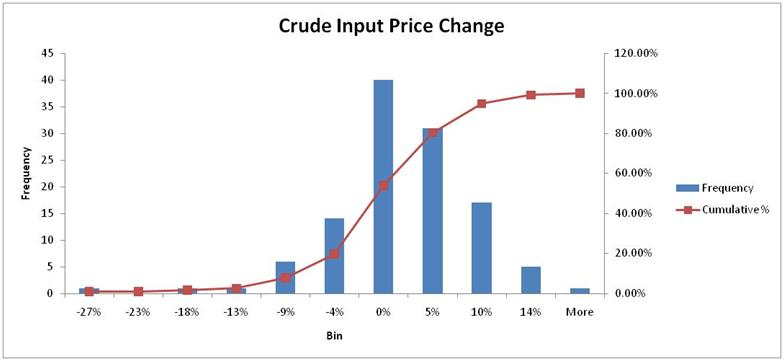
A distribution of returns is a tool that allows you to create and place a picture of your risk profile on your desk. Rather than looking at numbers you can actually see the shape of your exposure. For instance if you are exposed to the risk of changes in crude oil prices, the following distribution image shows what your risk profile has been like over the last five years on a monthly basis. In 60 months between 1st January 2005 and 31st December 2009, the most common month to month crude oil price change was zero%. The worst was -27%. The most was more than 14%. 90% of the month on month changes lay between the range of -9% and 10%. The shape of the distribution shows you that it is not symmetric and its worst case tail end lead to higher negative values even though the distribution as a whole is more skewed towards positive numbers.
Armed with the distribution we can use a number of interesting tools to assess what are likely risks numbers are. One such tools for measuring risk is Value at Risk (or VaR for short), a simple statistical technique that calculate a worst case loss, associated with a confidence level (think probability) and a holding period (think time horizon). The tool looks at the realized experiences (the historical distribution) and depending on the technique used, makes a number of assumptions about possible extreme deviations.
VaR’s most common representation is as a single dollar number that attempts to predict, given a fixed level of tolerance, the maximum loss that may occur on a portfolio over a given number of days.
In probability terms, tolerance is defined in terms of confidence level or confidence interval. This measure of tolerance incorporates the entire distribution of historical events, and specifies a fixed probability for the percentage of losses exceeding this predefined level of tolerance. Confidence interval is one of two parameters that form the basis of a VaR framework.
The second parameter for calculation of VaR is the holding period. If tolerance varies by institution, holding period will vary by portfolio. In a nutshell holding period for a given position should reflect the expected time the position will stay open or the number of days it will take to liquidate the position once a decision to exit is taken.
The following figure puts the above in context with some numbers. The 5 day holding period VaR calculated at 95% confidence level is the worst possible loss that may occur over the next 5 days, with a probability of being exceeded 5% of the time. Assuming that this VaR estimate is 1.5 million, there is a 95% chance that the actual loss realized over the next 5 days will be less than 1.5 million.
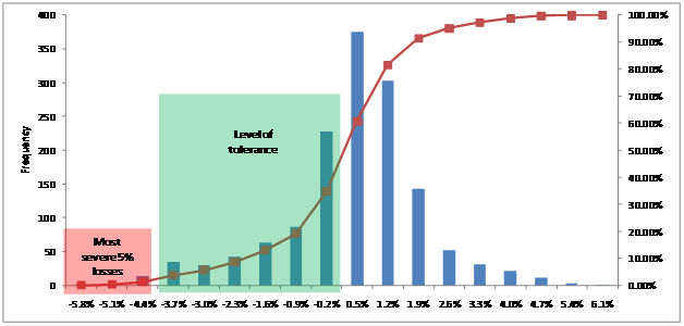
The chart above is a histogram of returns (think distribution) for a sample portfolio. The horizontal axis is used to plot the range of returns experienced on this portfolio, with the corresponding frequencies appearing on the vertical axis. The 5 tallest bars in the center represent the majority of returns. We can see that approximately 70% of the time the daily return was between -0.9% and 1.9%. The additional bars on the left and right represent very high gains and losses, but these have much lower frequencies.
The application of VaR ranges from risk measurement or estimating exposures, to capital allocation and risk control in the form of setting risk based trading limits and incorporating risk into pricing.
The first question that needs to be addressed is the level of application of limits. VaR based limits may be set anywhere in the hierarchical structure, from limits on individual traders, desks, business units or across the organization. The primary consideration here is the level of risk overlap between different risk centers. Once these limits are set, the control and monitoring process takes over (covered in the last section of this note).
Breaches in VaR limits may occur due to an increase in volatility, which results in an increase in the VaR numbers. This situation may be dealt with in two ways. The more conservative approach would be to adjust the limit immediately when a breach occurs. The second approach is to recognize that increase in volatility may be temporary, and set an acceptable band to accommodate temporary increase in volatilities before any changes to the limits are made. Of course the approach used to calculate volatilities can play a significant role. Volatilities calculated using simple moving averages tend to remain high till the observation that caused the spike does not drop out of the look back period. This problem may be addressed by moving to exponentially weighted moving averages where the weight of the observation decreases exponentially as we move forward. Irrespective of model used to calculate volatilities, temporary breaches in VaR limits due to sudden increase in volatilities may still occur and must be addressed.
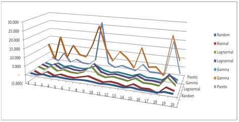
It is important to highlight the fact that like most quantitative finance and risk management models, value at risk has its limitations. VaR is not the maximum possible loss. VaR is simply an estimate to better understand the risk we are taking. In addition, this estimate is based on observed volatilities and correlations. The volatility over the next 10 trading days may differ significantly, and correlations may not hold. Finally two of the three VaR calculation models assume an underlying normal distribution as the distribution behind price behavior. The world as shown in the figure below is a bit more complicated than that.
While VaR used to be sufficient to quantify the required regulatory capital for trading portfolio, there is now literature questioning the effectiveness of this approach. The original critique of these models came through Nicholas Nassim Taleb (NNT) in a three part series in Derivative Strategies at the turn of the century where Taleb raised questions on the rationale behind using one number to describe the distribution. He took issue with the sense of false security provided by VaR based risk approaches, the breakdown of correlations under times of stress, the compliance driven mindset that led people to check off risk management once they had implemented an analytics and reporting system and the absurdity of assuming a Normal distribution for returns when we know the world is not Normal. This was followed by even more serious questions regarding impact of VaR platforms on overall market volatility and the increase in systematic risk rather than the expected decrease.
Taleb’s message focused on using risk profiles and price distributions over a period time to better understand the underlying risk distribution. This would only be possible if prices and volatilities tracked through time, if models were back tested, the right percentiles (lower) were used and expectations and incentives were set clearly and appropriately at the board and between risk takers and risk managers.
This course is based on the material presented in earlier editions of Pakistan Risk Review, the soon to be released Understanding Commodity Risk text book and the work done by Alchemy Technologies in the region in the area of financial risk management and Basel II reporting for the banking industry in Pakistan and the Middle East.
If you are looking for more coverage on understanding exposure to oil, its correlation with other commodities, the change in that correlation over time and possibly fair price of oil, please see the following sections
- Euro and Oil outlook – Trailing correlation between crude oil prices and Euro-USD exchange rates | Crude, Oil & Energy Insights
- Crude Oil price outlook – Is oil fairly priced now or still expensive. Or what can a barrel of oil buy – part ii | Crude, Oil & Energy Insights
- Crude Oil Trading – Trading USO | Crude, Oil & Energy Insights
- Crude Oil Price outlook – Detecting mispricing in precious metals and crude oil using trailing correlations | Crude, Oil & Energy Insights
Comments are closed.