While our generation of actuaries grew up with continuous time mathematics, my first exposure to actuarial functions and actuarial mathematics came through a chapter on commutation functions. A computational tool for easing the mathematics associated with repetitive calculations I grew so hooked to them that even today I use them as my first pass on a pricing function.
Commutation functions are a tool used by pricing and valuation actuaries. It is a means by which net single premiums and actuarial present values for various plans are determined. As compared to deriving these values from first principles, commutation functions once derived can be used to simplify and minimize the working that goes into computing these premiums, actuarial present values, etc. Through commutation functions intermediate values are tabulated and the premiums/values are expressed as functions of these intermediate values.
The commutation functions make use of the following as inputs:
- A life table which gives the values of lx at integer ages. lx represents the expected number of survivors at age x out of an original cohort of lives at some starting age.
- An assumption regarding a deterministic and constant interest rate per annum effective, i, that is used for discounting.
The commutation functions are defined below. Note that all summations (∑) go from y=x to ∞ (infinity):
Dx=νxlx ; where ν=1/(1+i) è discounted lives
Nx=∑ Dy = Nx+1+ Dx è sum of discounted lives
Sx=∑ Ny = Sx+1+ Nx
Cx=νx+1(lx– lx+1) è discounted deaths
Mx=∑ Cy = Mx+1+ Cx è sum of discounted deaths
Rx=∑ My = Rx+1+ Mx
The summations are given to infinity above. However life tables have values up to a finite maximum age. The actual calculations for the commutation functions therefore would terminate at the highest age that is present in the life table chosen.
Examples of how commutation functions are used to determined net single premiums, actuarial present values, etc. are given below:
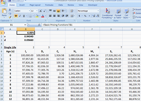
This is a screen shot of the hypothetical life table that we have used in building the commutation function table and the commutation functions derived in excel. Note that we have assumed that the interest rate, i, is 6% p.a.
The entries for x = 1, for example, are as follows:
ν = 1/(1+6%) = 0.94340
D1=ν1l1 = 0.94340*97957.83 = 92,413
N1= N2+ D1 = 1487613.81 + 92413.05 = 1,580,026.86
S1= S2+ N2 = 24266208.69 + 1,580,026.86 = 25,846,235.55
C1=ν2(l1– l2) = (0.94340^2)*(97957.83-97826.26) = 117.10
M1= M2+ C1 = 2860.47 + 117.10 = 2,977.56
R1= R2+ M1= 114054.82+ 2977.56 = 117,032.38
Life Insurance: Net Single Premiums
Ax= Net single premium for a whole life insurance paying a unit benefit at the end of the year of death to someone who is now aged x= Mx/Dx.
For a person aged 33 now, the net single premium for a whole life insurance paying 1000 at the end of the year of death is:
1000 * A33=1000*(M33/D33) = 1000*1624.44/13822.67 = 1000*0.11752 = 117.52
Ax:n= Net single premium for a n-year endowment insurance paying a unit benefit at the end of the year of death or at the end of the n-years whichever comes first, to someone who is now aged x = (Mx-Mx+n+Dx+n)/Dx
For a person aged 33 now, the net single premium for a 20 year endowment insurance paying 2500 at the end of the year of death or at the end of 20-years whichever comes first is:
2500* A33:20 = 2500 * (M33-M53+D53)/D33 = 2500 * (1624.44-1127.43+4001.66)/13822.67 = 2500*0.3255 = 813.642
IAx1:n= Net single premium for a n-year increasing term insurance payable at the end of the year of death to someone who is now aged x, where 1 is paid if the death occurs in the first year, 2 is paid is the death occurs in the second year, 3 is paid if the death occurs in the third year and so on = (Rx-Rx+n-nMx+n)/Dx
For a person aged 33 now, the net single premium for an 20-year term insurance payable at the end of the year of death, where 1 is paid if the death occurs in the first year, 2 is paid is the death occurs in the second year, 3 is paid if the death occurs in the third year and so on is:
IA331:20 = (R33-R53-20M53)/D33 = (48671.94-20734.44-20*1127.43)/13822.67 = 0.3899
Annuity: Actuarial Present Values
ax= The actuarial present value of a whole life annuity paying 1 per annum in arrears (i.e. at the end of the year), for life, to someone who is now aged x = Nx+1/Dx
For a person aged 60 the actuarial present value of a whole life annuity paying 100 per annum in arrears, for life is:
100* a60 = 100*(N61/D60) =100 *(25181.06/2482.16) = 100 * 10.144817 = 1,014.48
äx:n= The actuarial present value of an annuity paying 1 per annum for n years where payments are made at the beginning of the year to someone who is now aged x = (Nx-Nx+n)/Dx
For a person aged 60 the actuarial present value of a 20 year annuity paying 200 per annum at the beginning of the year is is:
200* ä60:20 = 200*(N60– N80)/D60 =200 *(27663.22-2183.49)/2482.16 = 200 * 10.2651 = 2,053.03
Iax= The actuarial present value of an annuity payable annually in arrears, for life, to someone now aged x of an amount of 1 in the first year, 2 in the second year and so on = Sx+1/Dx
For a person aged 60 the actuarial present value of a life annuity, payable in arrears, that pays an amount of 1 in the first year, 2 in the second year and so on is:
Ia60= S61/D60 = 223239.29/2482.16 = 89.9375