In this post, we continue with the definition of the calculation cells of the Black-Derman-Toy (BDT) model in EXCEL. Three state prices lattices are constructed.
The BDT model assumes that the short-term interest rates are log-normally distributed with risk-neutral probabilities of an interest rate going up or down in any time period of 0.5.
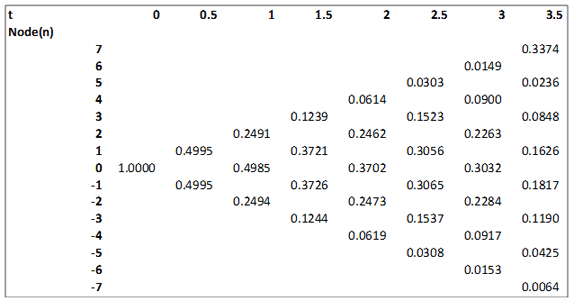
b.1. State Price Lattice for deriving price at node 0
At node n=0 and duration t=0, the price, Price0,0 is set to 1. At other nodes at duration t=0 the prices are left blank or set to 0.
At other nodes/ durations > 0 the price is:
Pricen,t= risk neutral probability × [ Pricen+1,t-1×exp(-rn+1,t-1×dt)+ Pricen-1,t-1×exp(-rn-1,t-1×dt)]
(Note that by t-1 we mean the duration one time step before t. For semi-annual compounding if t is 1 the duration t-1 is 0.5; for annual compounding if t is 1 the duration t-1 is 0)
For example the state price at node n=1 and duration 0.5 is (as per illustration dt = 0.5):
Price1,0.5=0.5×[ Price2,0×exp(-r2,0×0.5)+ Price0,0×exp(-r0,0×0.5)]
Price1,0.5=0.5×[ 0×exp(-0%×0.5)+ 1×exp(-0.21%×0.5)] = 0.4995
The lattice derived is as follows:
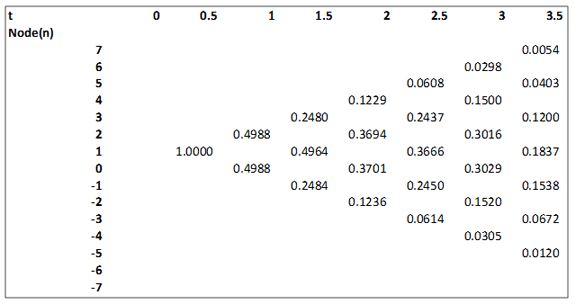
b.2. State Price Lattice for deriving price at duration 0.5 if prices were to move 1 node up(i.e. Price_up Lattice)
These shifted state price lattices (Price_up Lattice and Price_ down Lattice, details given below in b.3.) are needed to compute the prices if the user was now standing at duration 0.5 (assuming semi-annual compounding) instead of at duration 0. This in turn is needed for computing the volatility inherent in the short rate binomial tree.
The prices are calculated in a similar manner as given for the state prices lattice above (b.1.). Prices at all nodes at duration 0 will be 0. The Price at node n=1 and duration t=0.5, Price1,0.5 is set to 1. At other nodes for duration t=0.5 the prices are left blank or set to 0.
At other nodes/ durations > 0.5 the price is:
Pricen,t= risk neutral probability × [ Pricen+1,t-1×exp(-rn+1,t-1×dt)+ Pricen-1,t-1×exp(-rn-1,t-1×dt)]
(Note that by t-1 we mean the duration one time step before t. For semi-annual compounding if t is 1 the duration t-1 is 0.5; for annual compounding if t is 1 the duration t-1 is 0)
For example the state price at node n=3 and duration 1.5 is (as per illustration dt = 0.5):
Price3,1.5=0.5×[ Price4,1×exp(-r4,1×0.5)+ Price2,1×exp(-r2,1×0.5)]
Price3,1.5=0.5×[ 0×exp(-0%×0.5)+ 0.4988×exp(-1.15%×0.5)] = 0.2480
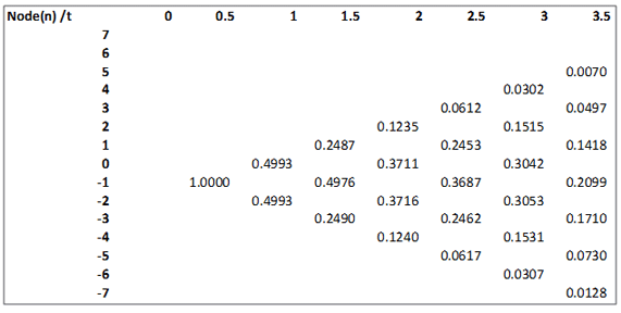
b.3. State Price Lattice for deriving price at duration 0.5 if prices were to move 1 node down (i.e. Price_down Lattice)
The prices are calculated in a similar manner as given for the state prices lattice above. Prices at all nodes at duration 0 will be 0. The Price at node n=-1 and duration t=0.5, Price-1,0.5 is set to 1. At other nodes for duration t=0.5 the prices are left blank or set to 0.
At other nodes/ durations > 0.5 the price is:
Pricen,t= risk neutral probability × [ Pricen+1,t-1×exp(-rn+1,t-1×dt)+ Pricen-1,t-1×exp(-rn-1,t-1×dt)]
(Note that by t-1 we mean the duration one time step before t. For semiannual compounding if t is 1 the duration t-1 is 0.5; for annual compounding if t is 1 the duration t-1 is 0)
For example the state price at node n=0 and duration 2 is (as per illustration dt = 0.5):
Price0,2=0.5×[ Price1,1.5×exp(-r1,1.5×0.5)+ Price-1,1.5×exp(-r-1,1.5×0.5)]
Price0,2=0.5×[ 0.2487×exp(-1.33%×0.5)+ 0.4976×exp(-1.00%×0.5)] = 0.3711
In this post we saw how state price lattices calculation cells of the BDT model were defined in EXCEL. The next post will cover how prices will be derived using the initial yield rates and these state price lattices.
Comments are closed.