Simulating Commodity Prices
Our course on Building Monte Carlo Simulators in Excel and related available-for-sale excel examples for Commodities, Currencies and Equities provide the groundwork for this EXCEL model. The model is an extension of the work done on this site as well as by us as part of our risk management practice.
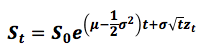
The traditional Monte Carlo simulation model generates future prices using the Black Scholes Terminal Price formula:
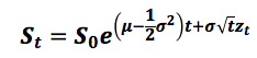
where zt is a random sample from a normal distribution with mean zero and standard deviation of 1. In EXCEL zt is obtained by normally scaling the random numbers generated using the RAND() function, i.e. NORMINV(RAND()).
The traditional Monte Carlo simulation model assumes that the underlying return distribution is normal. However, the question arises – “Does the normal distribution truly reflect how price returns actually evolve over time?” Let us consider the price return series for Gold. We have the following information and parameters available to us:
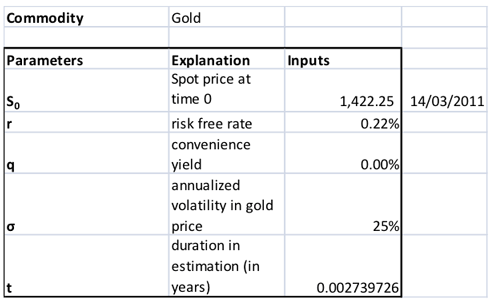
Figure 1: Parameters and inputs for the Monte Carlo simulation model
The spot price for gold on 14-March-2011 was 1,422.25. The one year US Treasury Yield curve rate on this date was 0.22% which we have taken as a proxy to the risk free rate. We have assumed a convenience yield of 0%. The average annualized volatility of actual price returns over the 365 trading day period from 15-March-2011 to 28-September-2012 was 25%.
Using the Monte Carlo simulation model with the Black Scholes Terminal price formula we simulate prices for the next 365 trading days. Note that µ is replaced in the formula above by the risk free rate less the convenience yield. The total period being considered is 365 days (=N) and the time step, t, is a daily time step, i.e. 1/365 expressed in years.
Actual price series against one scenario of the resulting simulated price series is given in the graph below:
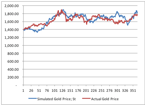
Figure 2: Actual Gold spot price series versus one scenario of MC simulated price series using the original approach
In this scenario, at first glance, the simulated price series seems to be fairly consistent with the actual gold spot price series. However, consider the histograms of price return series below. The histograms plot the frequency distribution of the return series:
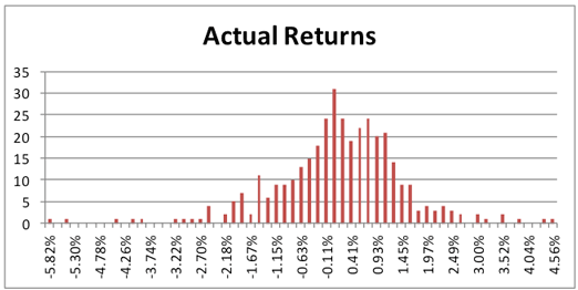
Figure 3: Actual Gold spot price return series histogram
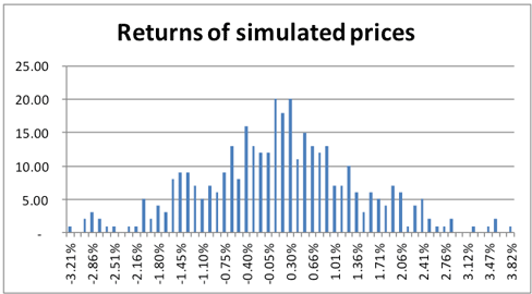
Figure 4: Simulated Gold spot price return series histogram using the original MC approach under one scenario
Actual returns show a much wider dispersion of returns and much longer tails than their normally simulated counterparts.
In another scenario, the prices series are themselves very divergent:
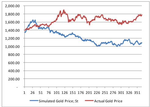
Figure 5: Actual Gold spot price series versus another scenario of MC simulated price series using the original approach
There is nearly a USD 700 difference between the actual and simulated price on day 365. And once again the normally simulated series do not capture the actual extreme tail events as can be since in the figure below:
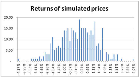
Figure 6: Simulated Gold spot price return series histogram using the original MC approach under another scenario
Average terminal price at day 365 over the following 25 scenarios show a difference of USD 300 between the actual price and the simulated price.
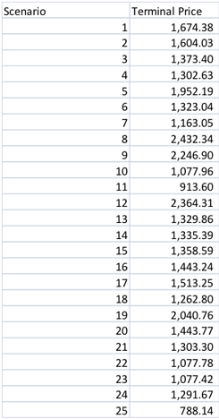
Figure 7: Data table of Terminal prices simulated for 25 scenarios using the original MC simulation approach
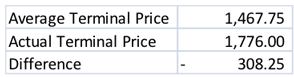
Figure 8: Average Terminal prices across 25 scenarios using the original MC simulation approach
In this chapter, we present an alternative method for simulating the price series to reconcile some of the difference that we see between actual historical and simulated returns. However, the important point to note here is that this method is a form of calibration of simulated results to historical returns. In reality, there is no guarantee that the future will pan out in a similar manner as it had done in the past. This is a necessary caveat or qualification that needs to be made if this model is used. If the future turns out differently from what has actually happened over the historical period of study being considered, results and decisions made on those results, may not retain their validity.
In the alternate method, the z-scores are determined from the actual historical return series rather than by applying the inverse of the standard normal distribution function in EXCEL to the random numbers generated using the RAND() function, i.e. NORMINV(RAND()).
To see how this is done let us once again look at the terminal price formula:
By rearranging the equation we have zt = (ln(St/St-1) – (r-q-o.5σ2)t)/σ√t.
Note that we have replaced µ with the risk free rate less the convenience yield, i.e. r-q, and S0 with St-1. The latter has been done because the simulated price path is determined using an iterative process where prices for that day, t, are derived using the previous day’s (t-1) simulated price.
The natural log of the ratio of successive prices, ln(St/St-1) is the daily price return at time t. If we replace this price return with the actual daily historical return, then zt will in effect be a derived z-score applicable to that historical return.
Each derived zt will be assigned an index number. This index number will be a multiple of 1/number of time steps, in this instance, 1/365. Why 1 in the numerator? Because the range between the minimum and maximum numbers in the uniform random series is 1. The first zt will be assigned 1/365, the second 2/365, the third 3/365 and so on.
In a variation to this method, the actual return series is then ordered in ascending order, smallest to largest and then assigned index numbers as above.
Random numbers are generated as in the original Monte Carlo simulation construction as discussed earlier, i.e. using EXCEL’s RAND() function. However, instead of normally scaling the random number, the random number is taken to stand for a particular index number. Using EXCEL’s VLOOKUP functionality the corresponding derived zt is then selected.
The rest of the model works in a similar manner to the traditional MC simulator, i.e.
- It calculates a path of prices, St, for each time step up to and including the Terminal price at the end of the specified duration, T.
- It uses N time steps, in this instance 365.
- It uses EXCEL’s DATA Table functionality to generate Terminal Prices for 25 different scenarios
- It calculates an Average Terminal Price from the results generated for the 25 scenarios
- It plots the path of prices & histogram of the distribution of returns for each scenario. By pressing the function key, F9, new scenarios are graphically displayed.
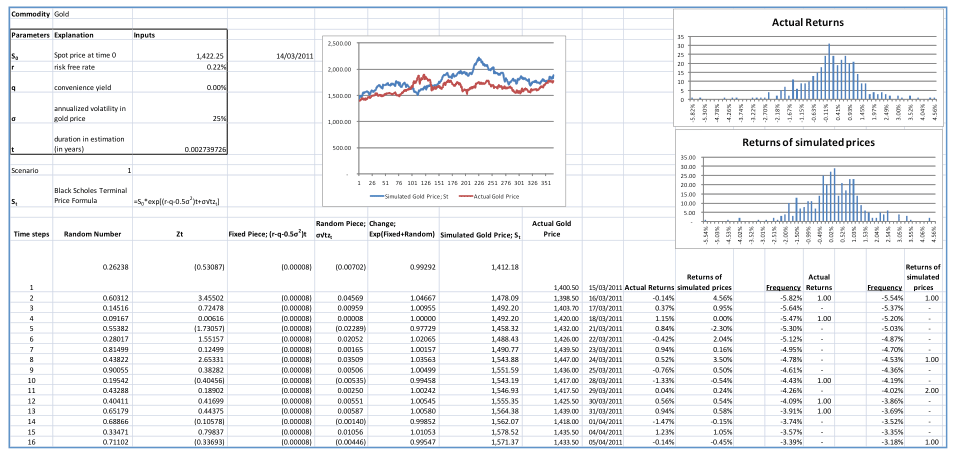
Figure 9: Monte Carlo Simulation model using Historical Returns
The scenarios generated under this alternative approach produce results that are more in line with the actual historical returns as can be seen from the price graph as well as the return histograms below.
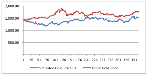
Figure 10: Actual Gold spot price series versus one scenario of MC simulated price series using the historical returns approach
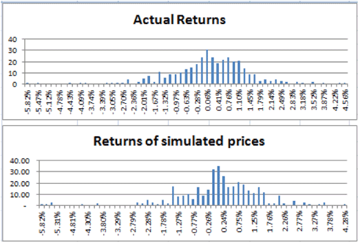
Figure 11: Actual versus Simulated Gold spot price return series histograms using the MC simulation with historical returns approach
Though there is variation in results from one scenario to the next these deviations on average are much less pronounced as compared to the original Monte Carlo simulation model. In our model, across the 25 scenarios captured in the Data Table, the average of terminal prices converges more closely to the actual spot price of gold on 28-September-2012:
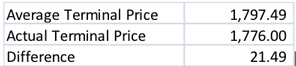
Figure 12: Average Terminal prices across 25 scenarios using the MC simulation with historical returns approach
Our MC simulator with Historical returns model for simulating commodity prices is now available for sale. To purchase the Excel file visit the Computational Finance section of our Finance Course Store.