Speeding up convergence. Using Quasi Monte Carlo & Antithetic techniques
In the past we have looked at Monte Carlo Simulation:
Computational Finance: Building Monte Carlo (MC) Simulators in Excel
We have also briefly touched on methods that may be used to improve the results obtained from this tool. These variance reduction procedures decrease the standard error between the simulated result and the true value as well as converge to the true result at a faster rate:
Monte Carlo Simulation: Convergence and Variance reduction techniques for option pricing models
In the following post we will further elaborate on these methods. In particular we will be looking at the Antithetic Variable Technique and the Quasi-random Monte Carlo method.
First however, we need to set the stage. We consider a European Call Option on a stock whose current spot price is 50. The strike price is also 50. The annual risk free rate is 5%, there are no dividends payable and the annual volatility in the underlying price series is 30%. The option will expire in 0.5 years.
Using the Black Scholes call option pricing formula we determine that the price of the European Call option is 4.8174.
We now use a one time-step or single path Monte Carlo Simulation model to simulate the option price. We execute the calculation for 100, 200, 300…, 1000 runs respectively. We then calculate the average value across the number of simulated runs to determine the estimated value of the option.
In the figure below we have plotted the results against the true Black Scholes result. You can see the variation of the results from the Monte Carlo methodology. This variation is also demonstrated in the magnitude of the standard error terms where standard error is calculated as the standard deviation of the simulated results (i.e. the sample) divided by the square root of the number of runs.


One way of improving the results is to increase the number of simulated runs considered. We can see this from the graph and table above. The accuracy for 500 hundred runs is greater than that for 100 runs while the result obtained after 1000 runs has a smaller standard error than the result after 500 runs. As the number of simulated runs increases in general the Monte Carlo simulated value converges towards the true value. Note however that as the number of simulated runs increases the computational time also increases. The other alternative is to use variance reduction techniques mentioned earlier where for the same number of runs the estimated value converges to the true value of the option at a faster rate and with a greater degree of accuracy.
Antithetic Variable Technique
Using this method we have actually doubled the sample being considered for the same amount of simulated runs. For each run we use the original Monte Carlo simulation results along with its negatively correlated result. These are averaged to obtain the result for a given simulated run under the Antithetic approach. This average series of results converges towards the true value of the option at a faster rate than the results from the original Monte Carlo simulation.
If the random numbers are generated from a uniform distribution (i.e. X~U(0,1) or RAND()), as is the case in our example, then the negatively correlated value is 1-X which is also uniformly distribution, (i.e. 1-X~U(0,1) or 1-RAND()). Alternatively if the normally scaled number from the original Monte Carlo simulation is Y, the normally scaled number from the second stream will be -Y.
We now have two parallel streams of random numbers that result in two sets of simulated prices, intrinsic values and values of options. For each simulated run take the average of the two options values to obtain the result for that run. The results for the Antithetic Variable method are given in the figure below:


If you compare the standard error terms above (calculated as mentioned earlier, i.e. standard deviation of the simulated results divided by the square root of the number of runs) with the error terms from the original Monte Carlo simulation method, you will see that they are much lower and that the convergence to the true value is much faster.
Quasi-Random Sequences. Halton sequence
Finally we use the Quasi-random Monte Carlo method to simulate the results for the value of the call option. Under this approach the random number series generated is actually not random at all but deterministic. We have used the Halton sequence which is a low discrepancy sequence which means that the samples points are more evenly distributed in the sample space.
Unlike a random number series where the data points tend to cluster together, the data points in this sequence are more uniformly distributed in the sample space as can be seen in the diagram below:

In our calculations because we have used only one dimension; the Halton sequence with prime base 2 will be used. What prime base of 2 essentially means is, we would keep on dividing segments into two portions. The line [0,1] is initially divided into two parts.
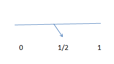
The division provides us with the first value of ½. If we had wished for a single value, we would have been done with this step. The next step is further dividing the segments into two more parts:
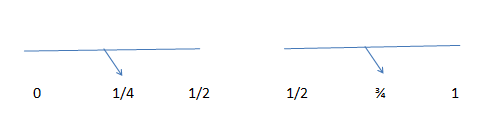
This gives a sequence of ½, ¼ and ¾. If we require more numbers we continue with the sequence generation:
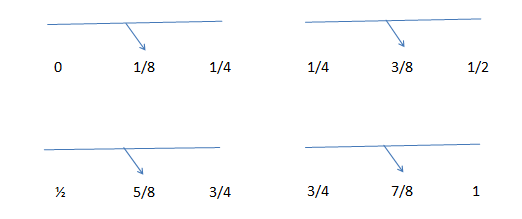
The sequence becomes, 1/2, 1/4, 3/4, 1/8, 3/8, 5/8 and 7/8. If the required number of sequence was 7, our work is complete. However, the sequences we would be dealing with will have values varying from 32 to 1024 so we will have to keep on dividing the values until we reach the required count.
This dividing into halves has prompted us to use number of runs as a power of 2. We had used base 3, we would have divided the line between [0,1] in third and would have repeated the process by dividing each individual segment into thirds again.
After normally scaling the values in this deterministic series we calculate the simulated prices, intrinsic values and values of option for each simulated run as we have done before for Monte Carlo simulation and the Antithetic Variable Technique. The results from the Quasi Monte Carlo method are depicted below:
As we have only used a single time step, i.e. one time interval in the sample path in our simulation, the dimension for the Halton sequence is one. Note that the Halton sequence has a different prime base for each dimension. For example, for dimension one the prime base is two; for dimension two it is three; for dimension three it is five, and so on. In our calculations because we have used only one dimension the Halton sequence with prime base two will be used.

Note that we have purposely kept the axis scales for all the graphs the same so that you can see the extent of the improvement in results. Compare the graph above to the earlier two. You can see that there is a significant improvement in the convergence rate of the results, in particular, in comparison with the original Monte Carlo simulation results.
The data points drawn from the Quasi-random sequence for each simulated run are not independent of each other as is the case for the Monte Carlo simulation and the Antithetic method, but are selected so as to more uniformly cover the entire sample space. Each subsequent number in the sequence is dependent upon the numbers that came before. Because of this dependency, the standard error term cannot be calculated as was done earlier for the original Monte Carlo simulation method and the Antithetic Variable Technique.
For a Quasi-random sequence method the best estimate for the standard error is the standard deviation of the sample divided by the number of simulated runs in that sample. The worst case or maximum error is the standard deviation of the sample times (ln(number of simulated runs)^dimension) divided by the number of simulated runs. The results are given in the table below:

References:
- Options, Futures & Other Derivatives, 7th Edition – John C. Hull
- Financial Risk Manager Handbook, 5th Edition– Phillipe Jorian
- Quasi Monte Carlo Methods in Numerical Finance – Corwin Joy, Phelim P. Boyle and Ken Seng Tan (Monograph –www.soa.org)
Comments are closed.