Credit Risk Models -Probability of Default

3 mins read

This is the first post in a multipart series on credit risk models. By the time we are done with this series, you should be able to calculate the probability of default for Barclays Bank (and if you really want, to calculate it for 4 other banks in the BBA USD LIBOR Panel).

PD Modeling using Merton’s structured approach

The essence of the Merton structured model is simple. The market knows best and knows it first before any of the analyst reports cover it. If you have a liquid publicly listed security, the price behavior of that security will be the first to indicate that something has gone wrong or is expected to go wrong. A valid, credible trade data signal is superior to an analyst research report.

But how do you best use market based signals? The Merton model is actually a variation of the Black Scholes model. Let us take a quick look at its intuition.

The valuation of firm equity as a call option on firms assets

We assume that the value of firm or shareholders’ equity is just like any other option. It becomes valuable as the firm grows and becomes less valuable as the firm declines. On one side of our balance sheet, the value of the firm is represented by its assets, which serves as a great proxy for how valuable the firm is. As long as firm assets exceed firm liabilities we are in good shape.

Equity is like a call option on those assets. While the value of liabilities of the firm is less than the value of its assets, firm equity has value. The minute value of liabilities exceeds the value of assets there is no incentive for the owner of firm equity to exercise the option. Rationally speaking the owner is better off simply handing over the firm to the bankers and walking away.

The Merton model for calculating the probability of default (PD) uses the Black Scholes equation to estimate the value of this option. The specification for this credit risk model is mapped as under:

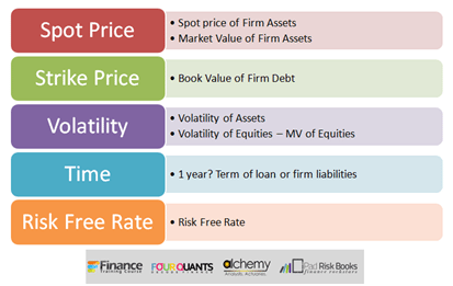
Credit Risk Models - Merton Structured Approach for calculating PD using Equity prices — **Figure 1 – Merton Structured Approach for calculating PD using Equity prices**

So we have:

Spot = Market value of firm assets,
Strike = X = Book value of firm liabilities,
Time = Term of liabilities.

However which volatility do you need? Firm Assets or Owner’s equity? The right answer is Firm Assets. However, we have a challenge. The observable volatility from market data is actually equity volatility. We, therefore, have to transform or convert it into firm assets volatility. Once that is done we have almost everything we need to calculate the probability of default.

a. Market Value of Firm Equity

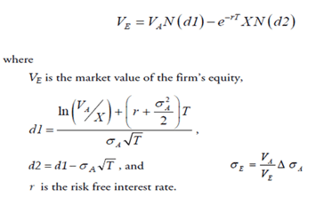
To make the transformation we need to estimate the market value of firm equity:

E = V*N(d₁) – D*PVF*N(d₂) (1a)
where,

E = the market value of equity (option value)
D = the book value of liabilities (strike price)
V = the market value of assets
T = the time horizon
r = the risk-free borrowing and lending rate
Sigma_a = the percentage standard deviation (volatility) of asset value
N = the cumulative normal distribution function whose value is calculated at d₁and d₂_,where:
- d₁= [ln(V/D) + (r + 1/2 sigma_a²)*T] / [sigma_a*(root(T)]
- d₂= d₁ – sigma_a*root(T)

In equation (1a), there are two unknowns: the market value of assets (V) and volatility of asset value (sigma_a). However, it is also possible to derive another equation from (1a).

b. Volatility of equity

Take the mathematical expectation of (1a) after differentiating both sides of the equations:

Volatility of equity (Sigma_e) = Function of (book value of liabilities, market value of assets, volatility of assets, time horizon) (2)

Again, this equation can be understood by using the Black-Scholes formula as an example. By taking the first derivative on both sides of (1a), and applying the expectation operator, one obtains the following expression:

sigma_e=[N(d₁)*V*sigma_a] / E (2a)

In equations (1a) and (2a), the known variables are the market value of equity (E), the volatility of equity (sigma_e, estimated from historic data), the book value of liabilities (D), and the time horizon (T). The two unknowns are the market value of the assets (V) and the volatility of the assets (sigma). Because there are two equations with two unknowns, a solution can be found.

Credit Risk Models - Merton Model Specifications - Simplified — **Figure 2 – Merton Model Specifications – Simplified**

c. Probability of Default

What is our estimate of the Probability of Default (PD)? Do you remember your Black Scholes analysis? What is the probability that ST > X? Is that what you need? In this case, default will occur when ST < X? What is the probability that ST < X? Our old friend N(-d2). That is your estimate for the probability of default.