Since we have a model for simulating oil prices, we are now ready to link our oil price model to projected financial statements for the airline.
To do this we need to figure out how to link simulated crude oil prices to jet fuel expense on the P&L statement. This means we need to determine:
- The correct correlation model between crude oil prices and jet fuel prices. If we don’t have a model we can start with a black box and refine later. The black box now, refine later approach will be used whenever there is a need to reduce complexity and move forward with the modeling process.
- The relationship between oil prices and demand or economic outlook. If a relationship exists that is great, if it doesn’t then we would need to build an independent model for economic outlook.
- A demand model for ticket sales (a combination of prices and volume based on oil price shocks).
Since we want to stay focused on modeling the process, we take a simplistic and direct demand model that will use oil prices to directly forecast ticket and cargo sales. Not an accurate approach but it will allow us to quickly test our model end to end. We also assume a perfect correlation between crude oil prices and jet fuel for our first pass.
Our simplistic demand model, looks at the change in oil prices and assumes growth or shrinkage in demand based on how high or low oil prices have moved as shown below. All the numbers below and the relationship between them have been picked out of thin air. In real life, we do a more robust job.
Monte Carlo Simulation – Building the demand model
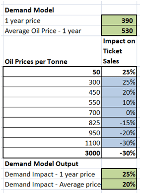
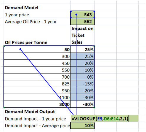
The two highlighted cells (50, 3000) serve as placeholders for the Excel VLOOKUP() function which is used to pick the applicable change in ticket and cargo demand based on where oil prices land in a given iteration.
Monte Carlo Simulation – Simulating Fuel Expense
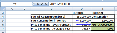
To simulate fuel expense a two step process is used.
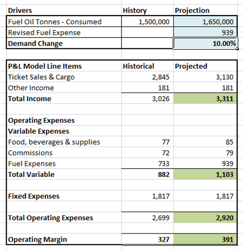
First using the simulated price, the cost of fuel consumed is estimated by using the new price and the old fuel consumption. In the second step, the number of units consumed are adjusted based on the projected change in demand. The two calculation are linked together to estimate the revised fuel expense as shown below.
The revised fuel expense is then plugged in variable expenses. Any additional variable expenses are linked to the demand (revenue growth) model and move accordingly. The same process is used for Ticket Sales & Cargo as well as for Food & Beverage and ticket sales commissions.
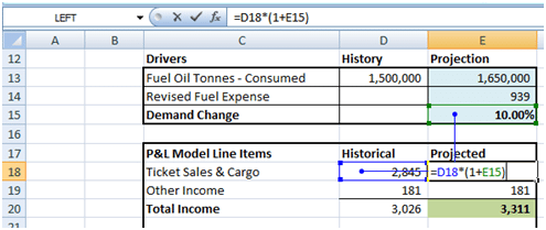
The final result is a simple simulation that allows us to model Operating Margin for the airline.
Monte Carlo Simulation – Storing the results
However, a single iteration of the model is meaningless. We need to use our old data table trick to store the results of the simulation in a data store which can then be used to calculate the average of our modeled variables over 500 – 5,000 simulations.
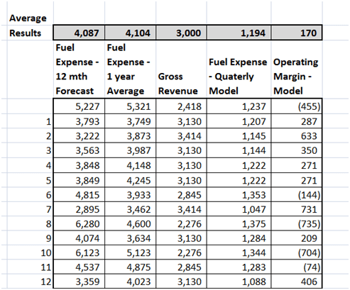
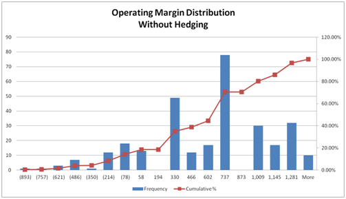
More importantly, the resulting data set can then be used to plot and generate a first pass for distribution of P&L (Operating Margin) for the airline.
Monte Carlo Simulation – Presenting the results
This model is by no means perfect. However a first pass can be put together in under an hour and as more data and analysis comes in, each of the black boxes (correlation, demand, ticket sales, etc) can be replaced by a more authentic and robust model. The most powerful output from the model is the P&L distribution. The distribution answers many common questions from Max Loss and Worst Case outlook to the probability that such scenarios will come to pass. It can also be used to evaluate hedge effectiveness across a range of possibilities. From testing the interaction of volatility and correlations to testing the demand model and the search for the right hedge ratio. Used correctly it can help you engage the Board productively as well as help the Board make a more informed decision.
Comments are closed.