In our first method presented earlier for calculating economic capital we used the historical worst case shift. In method two we use volatility. Method two is a variation designed to provide additional flexibility in estimating probability of capital shortfall in the event of market or regulatory intervention.
If you are comfortable with Value at Risk models, the first approach follows or uses the historical simulation model; the second follows the variance co-variance model.
Of our original seven steps, four steps remain the same. The new step is calculation of Shareholders equity volatility. Our mechanism for calculating distance to threshold and our approach to calculating economic capital also changes.
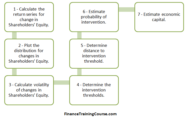
Step 3 – Volatility of Shareholders Equity
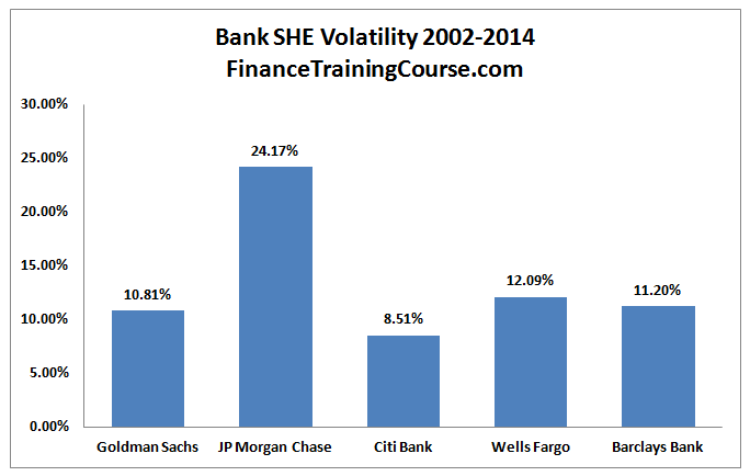
Calculating volatility of Shareholders Equity is a simple extension of our value at risk return series approach. We calculate the quarterly change from one quarter to the next. The series represents the percentage change. We then use the Excel standard deviation function on the series to determine the quarterly volatility figure. See the calculating return series for VaR tutorial). Multiply the result by square root of 4 to get an annualized volatility estimate and we end up with the series shared below.
Step 4 – Determine the intervention threshold
The intervention threshold remains the same as method one. From a capital adequacy perspective this threshold has been set at 10%. When a bank fall below the 10% threshold, model expectation is that either the regulator or market forces will react and intervene.
Step 5 – Determine distance to intervention threshold.
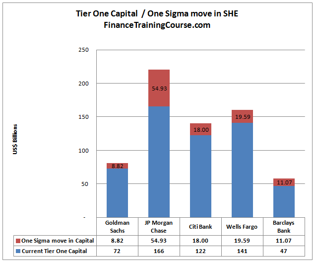
To estimate the distance to threshold we need to translate our annualized volatility estimate to an absolute annual amount. This is the amount that will reduce Shareholders equity in the event of a worst case loss.
We express these losses in terms of volatility. A one sigma loss is the current shareholders equity balance multiplied by one unit of volatility. A two sigma loss is two standard deviation, three sigma is three. The chart above expresses these losses in terms of one sigma shock. A shock that is within the range of a single standard deviation move in Shareholders equity.
Distance to intervention threshold is also measured using sigma moves. To calculate it, we refer back to our minimum regulatory capital threshold calculations to determine our estimate for excess regulatory capital stock.
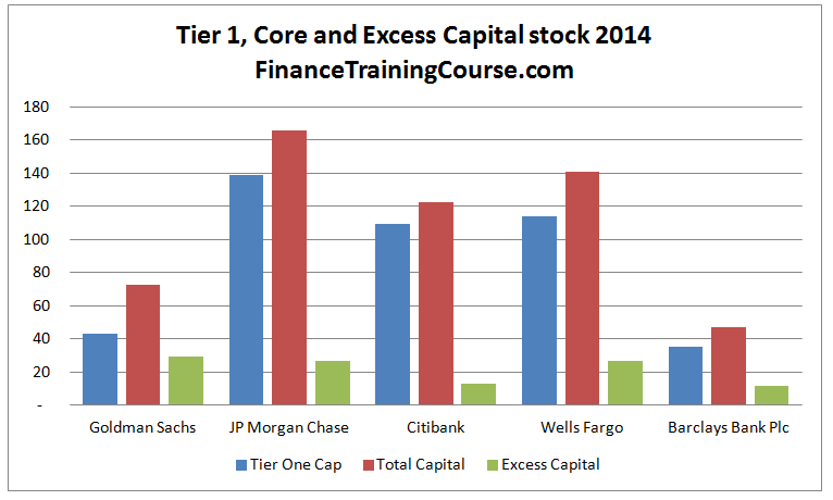
Armed with the original excess regulatory capital figure we estimate the number of sigma moves need to wipe out the excess capital buffer. Remember as per our model intervention happens not when the capital is completely utilized but as soon as the bank in question falls below a regulatory or market intervention threshold.
While Citi and Barclays have received more than their fair share of coverage, a number of market participants would believe that JP Morgan Chase and Wells Fargo are safe banks when compared to the likes of Goldman. We were just as surprised by the results of Model One but we internally justified that anomaly by the recent hits taken by JP Morgan Chase on account of London Whale. Our second model is less impacted by extreme scenarios and more by average volatility. Will the same results still hold? Or will we see a different trend when it comes to these five banks.
The next graph presents our model results. Here is how you should read it. The higher the blue line, the safer the bank in question is in terms of capital adequacy. So Goldman does very well by that standard. The other four are more or less in the same category but surprisingly Citi is rated higher than JP Morgan Chase.
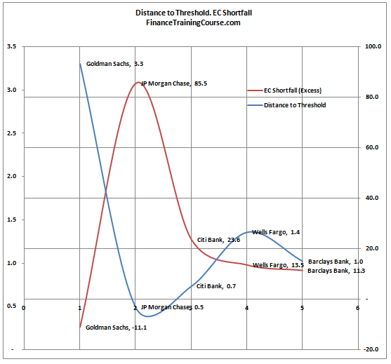
The higher the red line, the more capital the bank in question needs. Once again Goldman does well by this standard and JP Morgan Chase is once again ranked the lowest of the lot.
How do you translate these results to probability of intervention? Remember here intervention does not mean default. It means that you are now likely to be on the receiving end of either a regulatory intervention or a market based intervention. A regulatory action is generally more smoother and to be successful must work at the speed of a lightning strike. However there have been instances where the strike has gone south.
A market intervention is essentially a run to the exit by counterparties and tends to be disorderedly and chaotic. If the bank is large enough, it can create ripple effects that traverse the globe.
We apply a simply NORMSDIST function to the distance to threshold to assess the probability of such a move. The results are shared below:
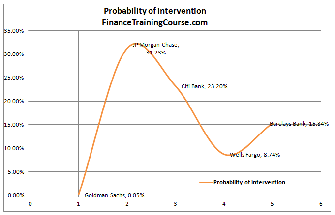
Once again Goldman does better by this standard amongst the lot and JP Morgan is ranked the lowest.
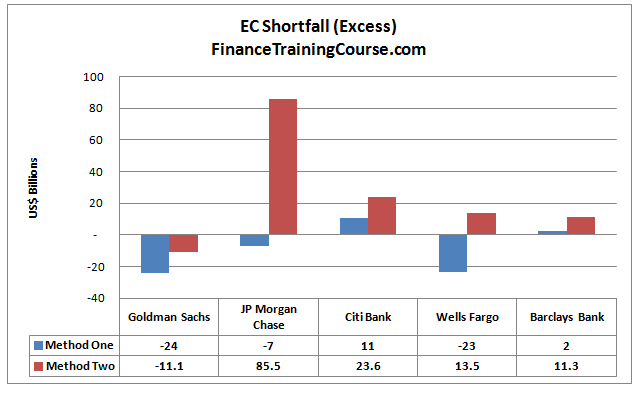
While probabilities are nice, if we were to compare apples to apples and not oranges it would be useful to compare the results for economic capital requirements across the two approaches (models). More so since method one is a little restricted when it comes to calculating probabilities. Here are the results:
Reconciling the difference in results for the two approaches.
There is a reason for the significant difference in Economic Capital estimates for the two approaches across our universe of 5 banks. Model one works with a worst case loss estimate and assumes that the threshold for Economic Capital is set equivalent to 3 worst case losses that occur in a sequence. Model two works with estimated volatility and assumes that a distance to intervention threshold of 3 (expressed in terms of shareholders equity volatility) provides sufficient protection. Model one works with the true underlying distribution, model two assumes normality when it estimates distance to intervention threshold.
Given how our data set is structured the probability of such an event occurring (3 consecutive worst case losses) is 0.00085%. Alternatively it corresponds to a confidence level set at 99.99915%. We can try and calibrate method 2 using this approach by using 4.3 as a required distance to threshold rather than 3.0 in our model.
An alternate approach to is to use model one with a required distance to threshold of 1. This implies a single worst case loss. This represents a probability of occurrence of 2.04% and a Z-score of 2.05 which we can use in model two. When we plug in the two numbers in our models the results are still quite different from each other.
As per model one, other than Citibank and Barclays, all banks in our dataset are reasonably capitalized from an Economic Capital point of view. Citibank and Barclays need an additional injection of capital. As per model two, other than Goldman, all banks need a significant injection of economic capital.