We use a simple illustrative example to show how to use Key Risk Indicators (KRI) and Loss Events to estimate operational risk capital associated with a given risk.
RCSA results. Computer failure: – Our RCSA exercise has determined a number of Key Risk Indicators (KRI). One of the key KRI is Number of Computer Failures per month. Given the abundance of logs and monitoring systems we also have the data for such failures.
KRI and its relation to Loss: – Develop a relationship or map between KRI and its impact on business lines and operations to understand the impact and how it creates risk for the bank.
Number of computer failures per month needs to be quantified in dollar terms. Our RCSA exercise also indicates that the primary issue with computer failure is unsuccessful transactions. Transactions unable to post, commit or close because the underlying computer component has failed. This ranges from transaction failure at ATM networks when a customer is attempting to execute a function, to a treasury systems transaction failing to post, leading to issues at day end or during central bank reporting because of a failed transaction that the bank did not identify, rectify or correct.
To understand the relationship between this specific KRI and a given scenario we can use conditional probability to estimate the number of unsuccessful transactions that the bank did not identify, rectify or correct in time and that occur because of computer failure.
Loss Data: – Based on frequency and severity estimation using loss data from our system logs we can drill down to specific transactions and loss in dollar terms for that given KRI.
Capital Estimation Model: – Collate loss data for all KRI’s and then group by business lines. Use aggregation of this data to estimate capital for Operational Risk.
KRI Loss Event Capital Estimation case study
Goodman Bank has setup a new Operation Risk management department. The first task is to find out potential processes, practices and activities which could lead to a risk. Then, to find ways of risk assessment and control. In order to do that we use Risk Control Self Assessment (RCSA).
Our Op risk management team identifies ‘Server Outage’ as one of the KRIs which could lead to potential loss. The head of ERM department needs to develop a model explaining how this KRI affects operational risk capital estimation.
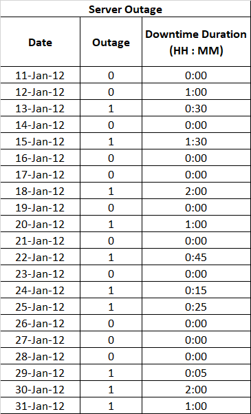
We start with finding data regarding server outages from the IT department. A list with Server Outage details on daily basis, for the last 100 months, with the duration of server downtime is below.
Relation between KRI and loss event
We understand that server outage can lead to a risk event. However, we do not find a direct relation with loss itself. Keeping this in mind, we look for a identified KRI and an associated event that can lead to a loss.
We look into different processes across the RCSA entities. And find that failed (incomplete) transactions that we did not catch, identify, report and fix in time can be a possible server outage related event. In order to confirm our initial assessment we look for daily data related to failed (incomplete) transactions from the treasury trading and sales department. The reason for using treasury department data set and servers is that unlike core banking and ATM network failures, we actually have a closed system within which the impact of a failed transaction can be easily quantified in dollar terms.
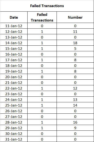
In this table 0 and 1 denotes occurrence of fail transactions for a given day. To develop a relationship between failed transactions and server outages, we need to see what the probability of failed transactions occurring is given that there is a server failure or outage.
Conditional probability
To calculate the conditional probability, we build another table. This gives both failed transactions and server outage over a span of sixty day. We add a column called the ‘Joint’ [failure]. It takes a value 1 when there is a failed transaction with server outage; and a value of 0 if none of the events take place. The table with sixty days data is below.
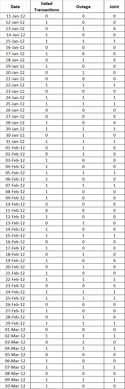
With the help of the table we can compute the probability of failure of transaction given there is a sever outage or failure.
The total number of possible outcomes: 60 (i.e. no. of days)
FT – Number of days with failed transactions: 35
SF – Number of days with server failure/outages: 28
FT SF – Number of days when both occur: 17
Determine the probabilities for above events by dividing each one of them with total possible outcomes. This gives us .58, .46, .28 for FT, SF and FT SF combined respectively.
Once we know the marginal probabilities for all three events, we find the probability of transaction failure given that there were server failure/outages. We use the conditional probability formula as follows:
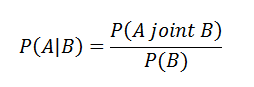
Writing in terms of SF and FT and calculating:-

This shows that 61% Transaction failures are due to Server Outage or failure.
Risk Scenario and Loss Data
Now that we established a link we now need to quantify the losses in dollar terms.
After some investigation, we find the loss data associated with failed transaction on daily basis. Within the treasury system failed transactions take many forms of loss. We highlight two such instances below:
- A failed limit update leads to a counterparty limit breach which is caught at day end and leads to the day end process being delayed. The delay leads to a vendor support call which incurs a charge at the out of office overtime rate of the vendor. In addition the treasury desk and the IT support group works for an extended operating time.
- A failed transaction post leads to incorrect execution of a market transaction that has to be rolled back and re-executed at different market rates than committed to a counterparty. Consequently, this may leave the bank with a mark to market loss on both ends of the transaction (roll back as well as re-execution).
The table of loss data collected from the treasury system follows:
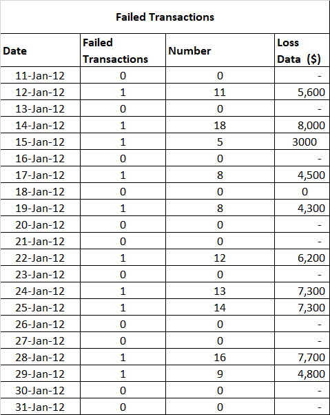
The loss data varies on a daily basis and its value depends on the number (frequency) of failed transactions. Based on the conditional probability, we can find the average value of losses due to server outages over a period of month. This gives us an estimate of the loss amount which is due to the server outage/failure.
By following this approach, we make a monthly loss data table for the last 100 month based on the daily data.
Capital Estimate and Observations
Estimate the capital requirement using on the loss data and the loss distribution approach.
Construct a histogram for the loss data for 100 months as below:
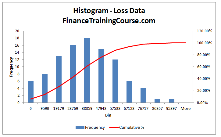
Figure 1: Loss data for the 100 months period represented by a histogram and a Cumulative Distribution Function (CDF) for the data set.
From the histogram we see that the data represents a normal distribution. To further investigate this we determine a probability plot using regression analysis in EXCEL. The probability plot is as below.
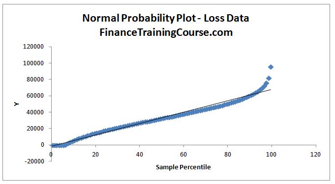
Figure 2: Normal Probability Plot for the loss data
From the probability plot, despite some outliers, we can safely assume that the normal probability distribution is a good fit.

References:
- Jan Lubbe and Flippie Snyman, “The advance measurement approach for banks”.
- Nigel Da Costa Lewis: “Operational Risk with Excel and VBA”, John Wiley & Sons .
Comments are closed.