Copulas in Excel. Theoretical foundations.

5 mins read

Copulas – revisiting the definition.

In our first lesson on Copulas in Excel we introduced the concept of marginal (individual) distributions for the two blends of crude oil we are interested in modeling. We also spoke about a joint distribution for a portfolio comprised of the two blends. It is now time to dig a little deeper.

Copulas are used to determine the joint distribution for different assets returns or portfolio risks while maintaining a stable correlation between the two variables. Imagine the need to model or simulate portfolio returns on a portfolio that includes two blends of crude oil, WTI and Brent; Or some combination of precious metals, Gold and Silver; or a mix of two currencies, Euro and Yen.

We could assume zero correlation between the two securities and use two independent distributions for the two positions, run a Monte Carlo simulation and combine the results. This would be factually incorrect because we would be assuming zero correlation and that may not necessarily be the case. Also because of the nature of the simulation, each simulation run would lead to a different correlation estimate.

You could also use a single correlation value between the two securities using historical data and use a value from your random distribution for WTI to calculate the corresponding value for Brent; from Gold to Silver or Euro to Yen.  In this specific instance you would no longer assume independence between the two distribution but a direct relationship modeled by your dependence or correlation variable.  But you would need to build a model that would generate corresponding values of the second security (Brent, Silver, Yen) in your portfolio for every value of the first security (WTI, Gold, Euro).

A copula is a tool that allows us to manage the above process.

Think of a copula as a transformation map that allows you to model the relationship between two securities, processes and phenomenon. We have only used financial instruments here so far in our examples but you can very easily use copulas to model the relationship between credit risk exposures and operational risk losses, number of teller transaction and central bank penalties, network load and ATM failures, custodial account growth and class action law suits, number of branches and customer complaints.

Let’s took a closer look at these tools.

Introducing Frank and Clayton

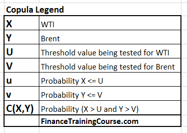
We started our discussion with two securities (X,Y) and we will stay with them through the presentation. You can read the (X,Y) combo as (WTI,Brent) or (Gold, Silver) or (Euro, Yen).

We also have F₁(X) and F₂(Y) which are the marginal (individual) distribution functions for the two securities whose returns we are trying to model. F1 and F2 could represent Normal, Lognormal, Beta, Gamma, Uniform or even a customized distribution function that generates a value or return for the security in question.  Using the context above we would denote these distributions as F1(WTI) and F2(Brent).  Where F1 and F2 would be the respective marginal distributions for WTI and Brent.

The combined joint cumulative distribution for the two securities is represented by C (F₁(X), F2(Y)) or C(F1(WTI), F2(Brent)).

Frank and Clayton Copula

Our modeling relationship takes two possible forms. Frank or Clayton copulas.

Starting with the Frank Copula, the Frank copula is given by the following formula:

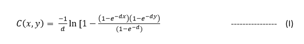
Remember X=WTI, Y=Brent, d is the dependence between the two securities, e is the exponential function and C(x,y) is the joint distribution.

The above equation can also be written as (by taking anti log and re arranging):

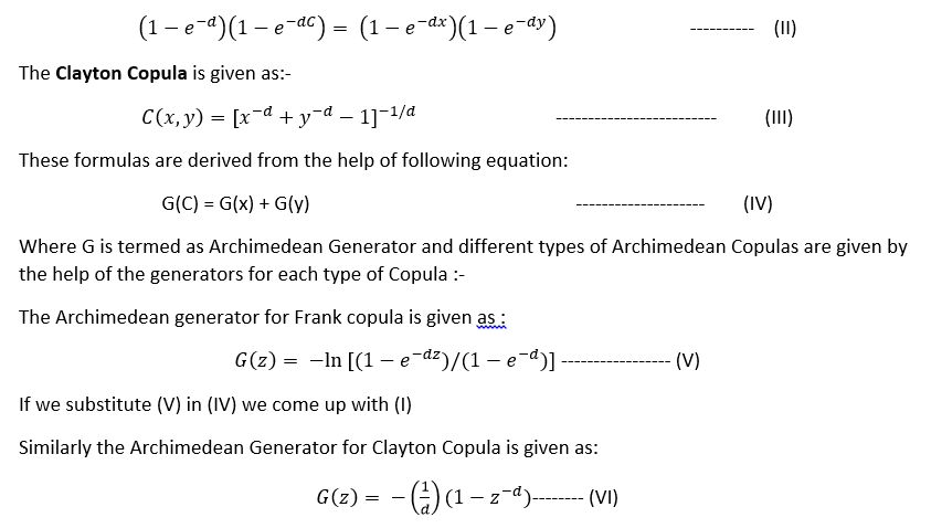
Substituting (VI) in (IV) gives us (III)

The C(x,y) function given for both the copulas satisfy all the properties for copulas.

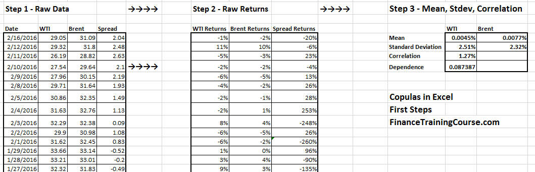
Building Copulas in Excel for WTI and Brent

We now have two sets of data which is price series for the two crude oil blends, WTI and Brent. We have also calculated their daily returns and estimated mean, standard deviation and correlation. We know that the value of X and Y might not lie in the range [0, 1]. But the cumulative distribution function F₁(X ) and F₂(Y) will lie on interval [0,1] (because by definition the probability distribution can only hold a value between 0 and 1).

Now let’s say for a given value of X, say U we need to find probability that X <= U and similarly for given value of Y say V we need to find probability that Y<=U , these probabilities will be given by F₁(U) and F₂(V) respectively.

The joint probability for the above two events (i.e. X<= U and Y<= V) will be given by:

F (U,V) = C(F₁(U), F₂(V)) , —————– (VII)

What we understand from (VII) is that a joint distribution function for U and V can be calculated by the help of individual marginal distributions if we select some Copula C.

Irrespective of the shape or form of the joint distribution there will be a Copula which will satisfy the above equation.

Let us also introduce v and u where u = F₁(U) and  v=F₂(V), and where u and v will also lie on [0,1] interval, and u and v will be uniformly distributed since they are probabilities.  Further if the probabilities are given we can calculate U and V by the help of the inverse function.

If we write (VII) in terms of u and v it can be written as

C(u,v) = F(F₁^-1(u), F₂^-1(v)) ———– (VIII)

This equation gives us the uniformly distributed variables we were looking for and now we can simply do the modelling by the help of the random function in Excel (rand()). Given that we know the mean and standard deviation for the time series (i.e. WTI and Brent daily returns or percentage price changes in our case).

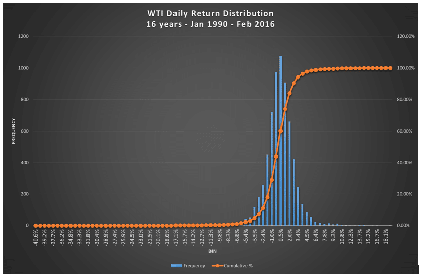
If we look at the histogram of returns for the two crude oil blends, we will see that we have slightly skewed distribution, somewhere between normal and lognormal.

We can obtain the value of u by taking the cumulative distribution function of x which will give a uniform value on the [0,1] interval. Similar procedure can be done for Y and value of v can be obtained.

If we plot v vs. u we will get a plot which will lies in the [0,1] interval. On the other had we can also plot NORMSINV for x and y which is more meaning full for the time series data. For both cases the correlation remains same and doesn’t affect the result.

Once more, just to ensure that we have complete clarity, here is the legend of the terms introduced so far.

One thing we need to understand that we have assumed that our series has an assumed normal distribution and we have obtained the values of x and y from the cumulative distribution function.

The Copula building process.

In case we are not sure about the distributions for the Copula and we have the mean and standard distribution for the time series under consideration we can use the following procedure.

1. Find the mean and standard deviation for both the series. (i,e, Stock X and Y)
2. Evaluate the probability that U<=X and U<=Y and hence the copula for v and u.
3. Generate a random probability for U<=x i.e. u=F(U) by the help of random function and find v in correspondence it by help of both Frank and Clayton copulas.
4. Frank Copula

From (I):-

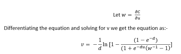
Differentiating the equation and solving for v we get the equation as:-

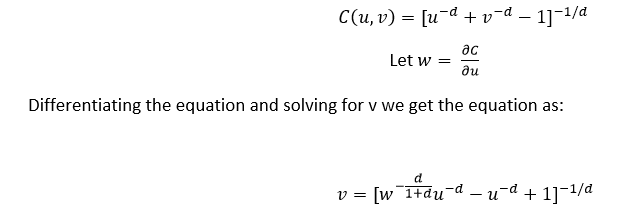
1. Clayton Copula

From (III):

1. We take the value of ‘w’ by the rand() function in excel.
2. Once we have the values of both u and v we use the NORMINV formula to get a distribution which is related to the mean and standard deviation of the data series we have and we term them x and y  for NORMINV of u and v respectively.
3. Once we have generated the data series we plot them in pairs on a graph which gives us both Frank and Clayton Copulas.
4. The Pearson Correlation can be calculated by the help of PEARSON function for the x and y data series.
5. We have also found out the ranks for the x and y series from which we can find the spearman relation between them.

In our next post we will walk through a step by step Excel example that follows this sequence of tasks.