Brent is the European crude oil blend. WTI is the North American pricing benchmark for crude oil. While Brent is used to price bulk of the crude oil cargoes purchased and sold across the world, WTI is the blend with the most liquidity in financial markets. If you want to buy physical cargoes you will most likely buy out side of North and South America using Brent. If you want to hedge your actual exposure using future contracts or options you have to work with WTI.
The range for the price spread between the two blends has been all over the place over the last sixteen years, the focus of our analysis. And modeling that spread is an interesting challenge when the spread has historically been as high as +30 or -30.
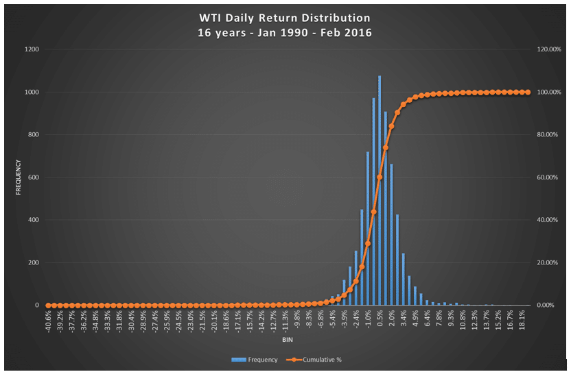
The first sign that this is going to be an interesting problem to solve is the histogram distribution that shows that while a large percentage of spread values over the last 16 years stay between -6 and +5, there are a number of extreme values on both ends.
When we dig a little deeper by plotting the value of the spread against a timeline we find that the distribution of spreads can be clearly linked to external geo-political events.
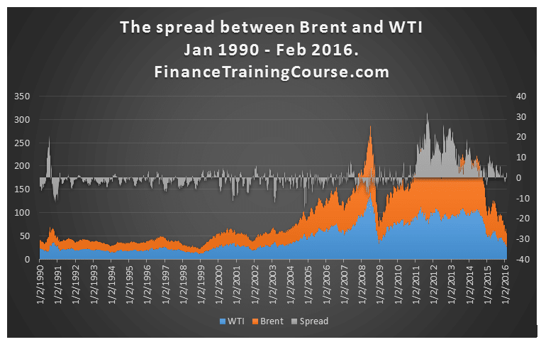
The graph above shows two clear and distinct spikes in the spread. Brent started trading at a premium in the events leading up to the first gulf war in 1990 and then again after the beginning of hostilities during the Libyan civil war of 2011. Post the oil price decline experiences beginning November 2014’s OPEC meeting, and the ensuing price war between Saudi Arabia (Saudi Aramco or AG), Iran (Iranian Heavy) and Russia (Urals), the spread between the two benchmarks has come down from its historical highs.
If we were to model correlation between the spread and the two blends, we will see quite a bit of model reversion, specially with correlation.
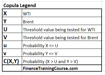
Using Copulas to model the spread between Brent and WTI.
The element we want to model using copulas in Excel is the spread between WTI and Brent. The first question is why use Copula’s for something which can easily be modeled using a simple regression model.
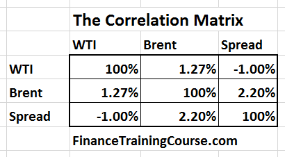
One look at the correlation matrix between the change in prices in WTI, Brent and the spread between the two should tell you that all is not well when it comes to modeling this relationship. One would assume that since oil is oil, crude oil prices should move together but they don’t. It won’t be possible to model the spread using a linear relationship such as linear regression.
We want to model the spread so that we can take the price of one blend and calculate the other. This requires us to model the price (or price changes) of both WTI and Brent and then use the modeled price to calculate the value of the spread at a given point in time. The implementation can be used in projecting costs of future cargoes or divergence between WTI linked hedges and our Brent linked purchase price.
Let’s try and see if we can use Copulas to solve this specific modeling problem.
The sequence of steps we would use to complete these tasks would be:
- Get data for WTI, Brent and the spread between them
- Calculate the return series for all three items
- Calculate the mean, standard deviation and correlations
- Apply Clayton Copulas to evaluate the values of X, Y, U, V, u, v and w
- Estimate d or the dependence variable
- Evaluate the fit between our model and actual historical results.
The first three steps are straight forward and were completed in our previous lesson.
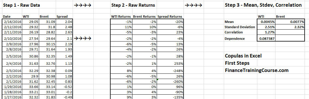
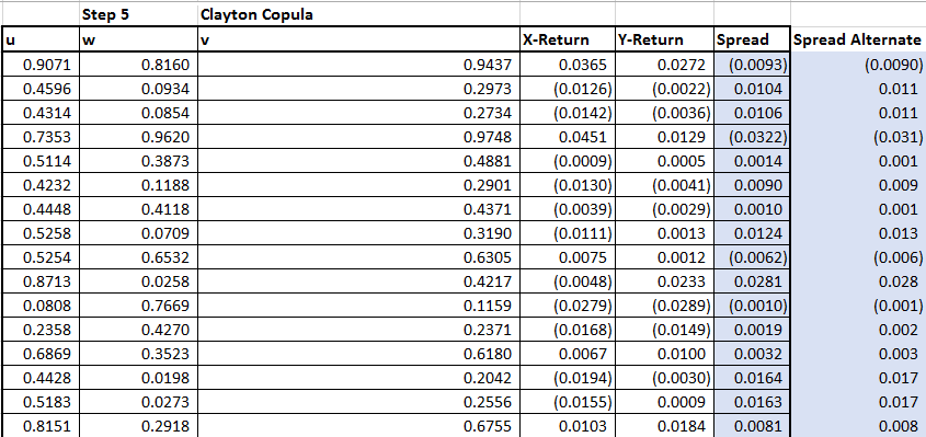
We move on directly to step 4 and calculate the values of X, Y, U, V, u, v and w using the Clayton Copula.
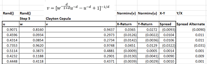
Where:
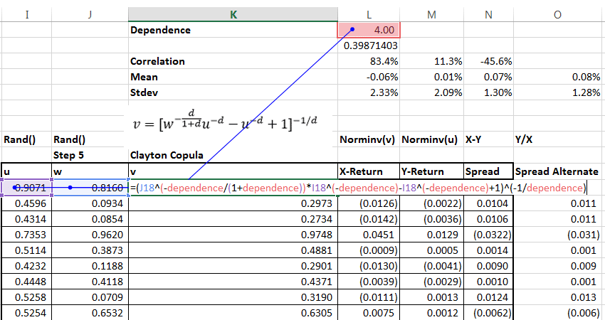
We start with calculating the values of u and w which are simple calls to the Excel uniformly distributed random numbers. Using u and w as our random seeds we calculate the value of v.
We then calculate X and Y using v and u as illustrated below. X and Y are simple Norminv calls in Excel
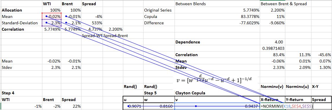
X and Y now represent our Copula implementation of the daily percentage return (change) in the value of WTI and Brent .
The highlighted series X – Y or X/Y is our representation of the spread between the two blends.
We then estimate the value of d or the dependence variable by iterating across values for d and keeping an eye on the independent series mean and standard deviation and the correlation between the change in the value of the spread and Brent.
The relationship between Dependence ’δ’ and Pearson Correlation ‘r’
When Archimedean copulas are used to model and understand the joint risk between two portfolios as part of Enterprise Risk Management for both the Frank Copula implementation we will come across the variable ‘δ’(it is also denoted by θ in some books) which is termed as the level of dependence.
This section explores the relationship between the correlation of two return series/time series and the level of dependence δ of Frank Copula.
In order to explain the relationship we have taken two return series of WTI and Brent as an example to help us in achieving the objective.
We have a return series for the both WTI (X) and Brent (Y) over a period of time from which mean and standard deviation for both the series is calculated. Let us call mean and standard deviation for WTI as mx and sx while mean and standard deviation of Brent can be termed as my and sy respectively.
For any value of δ we can generate the values for the cumulative marginal distributions u and v from the copula equation
We find the Pearson correlation ‘r’ for the series x and y. For our first iteration the value for our simulated series will not match the actual results from the original series being modeled.
This shows that the value of is not right as the correlation for x and y is not the same as the series X and Y. We can use different values of d and determine the correlation for it.
Also see theoretical foundations for building Copulas in Excel, Aggregating risks for ICAAP – Copulas at work and Building Copulas in Excel, the original post.
Additional readings: