This course presents a step by step methodology for building a one factor Black Derman Toy model in EXCEL.
STEP 1: Define Input Cells
In the following post, we consider the required inputs for the Black Derman Toy (BDT) interest rate model. These include among other things the initial yield rates and their volatilities. Other inputs are:
- the term of the instrument,
- the number and length of time step intervals considered,
- the valuation date, and
- the duration to each future node
STEP 2: Define Output Cells
Next, we will assign the output cells in the sheet. These cells will present the resulting values once we define the formula cells and link the solver function to them and run it. The outputs of the BDT interest rate model include:
- the median rates,
- sigmas (time varying volatilities), and
- the up movements or proportions by which prices increase. We use these movements in the construction of the BDT short rate tree.
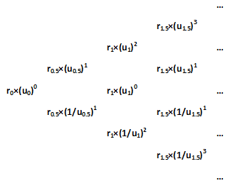
STEP 3: Construct a short rate binomial tree
In the next stage, we define the calculation or formula cells. The first step in this process is the setting up of the short rate binomial tree which we construct using the median rates, sigmas and up movements of the output cells:
STEP 4: Construct state price lattices
The next interim step is the construction of three price lattices. One derived at node 0, one at node 1 and one at node -1:
STEP 5: Calculate prices from lattices
We next define Prices- initial prices derived from the initial yield rates, and prices from each of the lattices defined in Step 4:
STEP 6: Calculate yields and yield volatilities from lattice
The final set of calculation cells involves calculating the yields from the lattice prices and then the volatilities from the resulting yields:
STEP 7: Define & Set Solver Function. Run Solver & View Results
The last step of the BDT interest rate model construction links the input, output and calculations cells together using the Solver Function. The Solver function is then run to arrive at the solved for median rates and sigma values:
Running the Solver function in Step 7 calibrates the model to the current spot yield curve and its volatility term structure.
An alternate method of calibration involves solving for the median rates and sigmas by minimizing the difference between the model and actual observed prices of very liquid instruments as of the valuation date. We illustrate this for US Treasury government bonds in the post below:
Workaround the limitations of EXCEL’s Solver functionality
EXCEL Solver functionality does have its limitations when there are a large number of adjustable cells. In such cases, Solver will fail to compute. In other instances even when the number of adjustable cells is within Solver’s capability, the function repeatedly returns an error or a message that it cannot find feasible results.
A workaround method is to utilize Solver in a piece meal fashion across the entire range of results. The post below discusses this methodology: