Forecasting the Monetary Policy Rate decision
Process
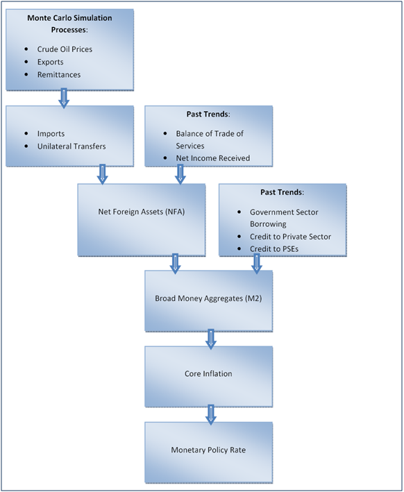
One way to look at the decisions on the monetary policy rate cut or rate hike is to look at simulating the rate of inflation in any economy. In order to determine what the inflation rate will be we use the underlying relationship between the Broad Money Aggregates (M2) growth rate and the inflation rate.
M2 numbers in turn are computed based on a number of elements. Our forecast model uses three primary processes to determine these elements. These involve simulation of future prices and amounts using a Monte Carlo simulator to determine:
- Crude Oil Prices
- Exports
- Remittances
Why oil? Primarily because in most emerging and developing economy Oil represents the biggest import and given the volatility in Oil prices over the last 3 years the most significant source of economic shock to an emerging or frontier market.
We use the underlying relationship between crude oil prices and imports to determine imports and the relationship between remittances and unilateral transfers to determine the amount of transfers.
These elements together with balance of trade from services and net income received, which are derived based on past trends, are used to determine the current account balance or change in the net foreign asset (NFA) of the country.
The change in NFA is used as an input for determining M2. Other principle inputs for calculating the M2 number, i.e. net government sector borrowing, credit to private sector and public sector enterprises, are based on past trends. M2 growth rates determine inflation rates as mentioned above, which are then used to calculate the extent of future policy rate cuts.
This process is depicted pictorially below:
Results
Step 1: Simulating Crude Oil Prices
The average crude oil prices for the months of July, August and September 2010 have been simulated using a Monte Carlo simulator.
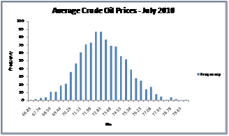
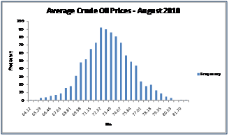
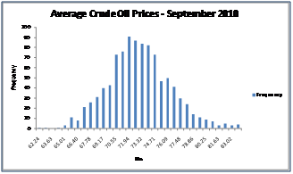
The best and worst case prices (per barrel) for July 2010 are USD 66.89 and USD80.05 respectively; for August 2010 are USD 64.12 and USD 82.28 respectively; and for September 2010 are USD 62.24 and USD 83.71 respectively.
Step 2: Calculating Imports
The historical relationship between imports and crude oil prices has been used to derive import figures for the first quarter of fiscal year 2011.
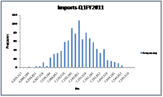
Historically average imports per month (over past 24-months) have been USD 2,624,764 (or USD 7,874,293 for three months).
The best case scenario under our model is USD 6,835,517 thousand of imports while the worst case scenario is imports of USD 7,620,852.
Step 3: Simulating Exports
The exports for the months of July, August and September 2010 have been simulated using a Monte Carlo simulator.
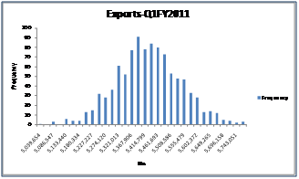
Historically average exports per month (over past 24-months) have been USD 1,630,212 (or USD 4,890,636 for three months).
The best case scenario under our model is USD 5,766,498 thousand of exports while the worst case scenario is exports of USD 5,039,654 thousand.
Step 4: Simulating Remittances
The remittances for the months of July, August and September 2010 have been simulated using a Monte Carlo simulator.
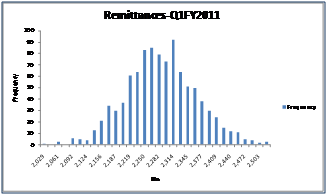
The best case scenario for remittances for the first quarter of fiscal year 2011 is USD 2,519 million whereas the worst case scenario is USD 2,029 million.
Step 5: Calculating the change in Net Foreign Assets (NFA)
The change in net foreign assets or the balance on the current account is based on the following inputs: exports, imports, unilateral transfers, trade balance for services and the net income received. Exports and imports are as derived above, unilateral transfers are based on the relationship with remittances and the latter two elements are derived based on their past trends.
The resulting increase in NFA falls in the range of USD 128.23 million and USD 949.57 million for the first quarter of FY 2011.
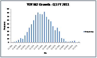
Step 6: Calculating M2 and M2 Growth
The change in NFA is used to calculate NFA for the period. The other factors that are used as inputs into deriving M2 are government sector borrowing, credit to the private sector and credit to public sector enterprises which are calculated based on their past trends.
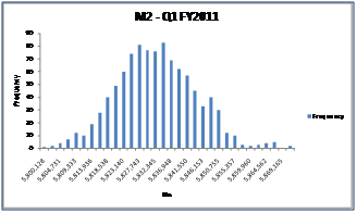
As at 30 September 2010 M2 aggregates are forecasted to stand between PKR 5,800 billion and PKR 5,871 billion which accounts for an annual increase of 11.78% and 13.15%.
Step 7: Forecasting Core Inflation
Using the historical relationship between annual M2 growth rates and core inflation the core inflation rates are derived.
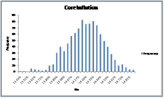
Under the best case scenario the core inflation rate is estimated to be 13.43% whereas under the worst case scenario the core inflation will be 14.85%.
Step 7: Calculating the cut in the policy discount rate
There is a relationship between the core inflation rate and the policy discount rate. Generally as inflation increases the monetary policy is tightened and the policy discount rate is increased. The opposite happens when inflation declines- the monetary policy is relaxed and the policy discount rate is cut. For the prior two cuts in the policy discount in August and November 2009, a minimum difference between the policy discount rate and the core inflation rate was maintained.
In the calculation of the cut it is assumed that a minimum difference of 0% is maintained and that there is no attempt made to further tighten the monetary policy (i.e. a policy rate increase is not on the cards)
Given the range of values for the inflation rate and the assumptions noted above the policy rate cut is 0% under all scenarios.