a. How to determine Forward Rates from Spot Rates
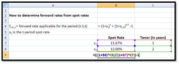
The relationship between spot and forward rates is given by the following equation:
ft-1, 1=(1+st)t ÷ (1+st-1)t-1 -1
Where
st is the t-period spot rate
ft-1,t is the forward rate applicable for the period (t-1,t)
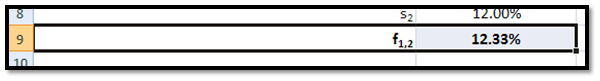
If the 1-year spot rate is 11.67% and the 2-year spot rate is 12% then the forward rate applicable for the period 1 year – 2 years will be:
f1, 2 = (1+12%)2÷ (1+11.67%)1 -1 = 12.33%
You may calculate this in EXCEL in the following manner:
b. How to determine Spot Rates from Forward Rates
Alternatively (and equivalently) the relationship between spot rates and forward rates may be given by the following equation:
For example you have been given forward rates as follows:
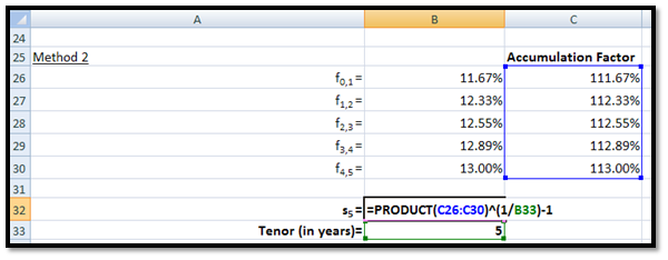
f0,1 = 11.67%
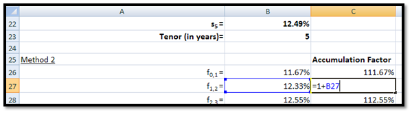
f1,2 = 12.33%
f2,3 = 12.55%
f3,4 = 12.89%
f4,5 = 13.00%
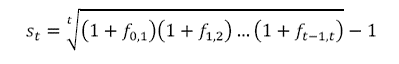
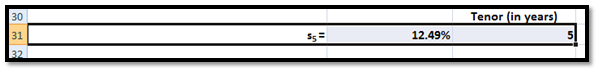
The 5-year spot rate, s5, will be:
[(1+11.67%)×(1+12.33%)×(1+12.55%)×(1+12.89%)×(1+13.00%)]1/5-1 = 12.49%You may calculate this in EXCEL in the following manner:
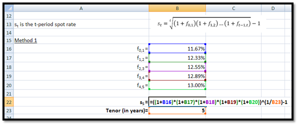
Alternatively you may first calculate accumulation factors, 1+f, for each forward rate as follows:
And then calculate the spot rate as follows:
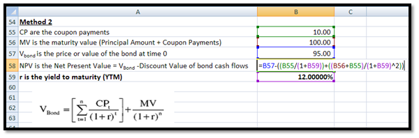
c. How to calculate the Yield to Maturity (YTM) of a bond
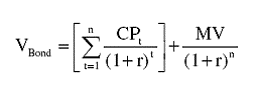
The equation below gives the value of a bond at time 0. The cash flows of the bond, coupon payments (CP) and Maturity Value (MV = Principal Amount + Coupon payment) have been discounted at the yield-to-maturity (YTM) rate, r, in order to determine the present value of cash flows or alternatively the price or value of the bond (VBond).
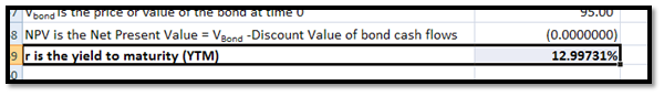
For example, you have a 2-year bond with face value (or principal amount) or 100 which will be paid at maturity, i.e. the end of the tenor of the bond. The bond pays an annual coupon at the end of each year of 10. The value of the bond at time 0 is given as 95. Putting these values into the equation above we have:
CP = 10
MV = Face Value + CP = 100 +10 =110
VBond = 95 =10/(1+r) +110/(1+r)2
This may be solved using a trial and error process or the equation may be solved for in EXCEL using the GOAL SEEK functionality.
i. Trial and error process for calculating YTM of a bond
1. Start with two points r= 0% and r= 15%.
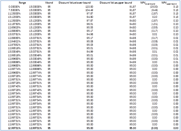
When r=0%, VBond– Discounted Value = Net Present Value (NPV) = -25.00
When r=15%, NPV = 3.00
Since one value is positive and the other negative the solution lies in the range 0% and 15%.
2. Half the interval. Consider r=7.5% and r=15%.
When r=7.5%, NPV = -9.49
When r=15%, NPV = 3.00
Again since one value is positive and the other negative the solution lies in the range 7.5% and 15%.
3. Again half the interval. Consider r=11.25% and r=15%.
When r=11.25%, NPV = -2.87
When r=15%, NPV = 3.00
Again since one value is positive and the other negative the solution lies in the range 11.25% and 15%.
4. Again half the interval. Consider r=13.125% and r=15%.
When r=13.125%, NPV = 0.20
When r=15%, NPV = 3.00
Since both values are the solution lies in the range 11.25% and 13.125% and not 13.125% and 15%.
5. Half the interval between 11.25% and 13.125%. Consider r=12.1875% and r=13.125%.
When r=12.1875%, NPV = -1.31
When r=13.125%, NPV = 0.20
Again since one value is positive and the other negative the solution lies in the range 12.1875% and 13.125%.
And so on till we arrive at the solution of r = 12.99731%. The complete list of iterations is given in the table below:
ii. EXCEL’s Goal Seek method for calculating YTM of a bond
First set up the input at output cells on the worksheet as follows:
Note that the value of r (the YTM) is initially a dummy value.
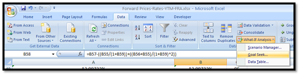
Next, set up the Goal Seek functionality. In the Data Tab, go to “What-if Analysis” menu and Click on Goal Seek:
Then enter the values in the Goal Seek pop up window as follows:
- Set cell = NPV
- To Value = 0
- By changing cell = YTM
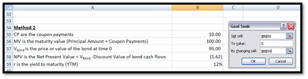
Click OK to solve for the YTM. The result is as follows:
As you can see Method 2 yields the same results as Method 1 (up to 7 decimal places) and is less cumbersome.