The Cox-Ingersoll-Ross, CIR, interest rate model is a one-factor, equilibrium interest rate model. One factor in that it models the short – term interest rate and equilibrium in that it uses assumptions about various economic variables (e.g. mean reversion) to derive a process for determining this rate.
We have already provided a detailed theoretical overview in the following posts of how CIR parameters may be calibrated and on how these resulting parameters may be used to simulate short-term interest rates and model longer term rates:
- Using CIR (Cox Ingersoll Ross) Model: Introduction
- Using CIR (Cox Ingersoll Ross) Model: Estimating Parameters & Calibrating the CIR Model
- Using CIR (Cox Ingersoll Ross) Model: Simulating the term structure of interest rates
CIR Interest Rate Model – Parameter Calibration & Simulation
In the following post, we will consider a practical example. Specifically, we will:
- Use the Daily Treasury Yield Curve Rates for the period 2-Jan-2009 to 27-Jul-2010 for our calibration exercise
- Calculate spreads between the short term rate as of 27-Jul-2010 with longer term rates for this date. These will be used later to model the longer term interest rates.
- Calibrate the parameters of the CIR model with the Simple Discretisation process
- Simulate the short term rates for the next 360 month period by using the derived parameters
- Use the spreads derived in Step 2 along with the projected short term rates in Step 4 to determine the long-term interest rates
STEP 1: Obtain the necessary historical interest rate/ yield curve data for CIR interest rate model
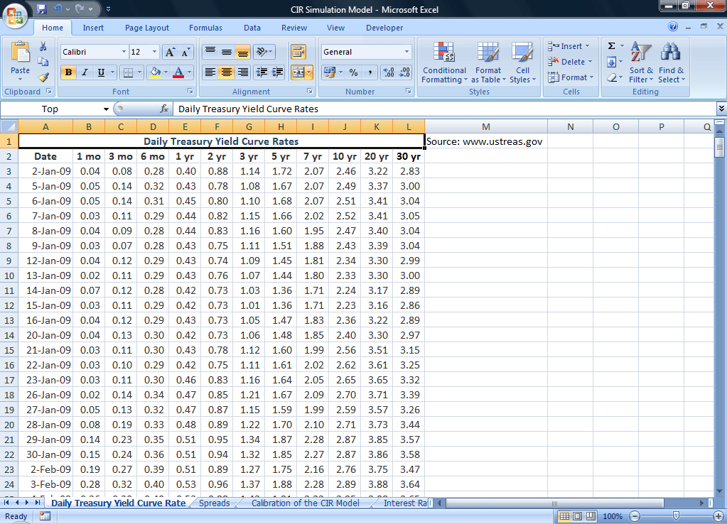
In order to calibrate the CIR interest rate model to our data set we first need to obtain the necessary data set. For our illustration, we have used the daily US Treasury Yield Curve Rates for the period 2-Jan-2009 to 27-Jul-2010 available at www.ustreas.gov.
STEP 2: Calculate Spreads for CIR model
Later on in this calculation, we will be simulating future short term interest rates using the calibrated CIR interest rate model. As an off-shoot to that simulation exercise, we will also be modeling longer term rates. These longer term rates will be a function of the projected short term rates and historical spreads. For simplicity we will be using spreads for a single day, i.e. 27-Jul-2010, but the user may choose to base his/her calculations on average spreads over the selected period instead.
For 27-Jul-2010 the interest rate term structure for US treasury rates was as follows:
| Tenor | 27-Jul-10 (%) |
| 1 mo | 0.16 |
| 3 mo | 0.15 |
| 6 mo | 0.21 |
| 1 yr | 0.30 |
| 2 yr | 0.65 |
| 3 yr | 1.02 |
| 5 yr | 1.82 |
| 7 yr | 2.51 |
| 10 yr | 3.08 |
| 20 yr | 3.88 |
| 30 yr | 4.08 |
We first determine the interpolated rates for each month from 1 month to 360 months (i.e. 30 years). For instance, the 2-month interest rate will be interpolated using the 1-month and 3-month rates.
2-month rate = [(2-1)*0.15%+(3-2)*0.16%]/[3-1] = 0.31%/2 =0.155%
Next, we determine the spread between this interpolated rate and the short rate (i.e. the 1-month rate) = 2-month rate – short rate =0.155%-0.16%=-0.005%.
A snapshot of the resulting rates and spreads is given below:

STEP 3: Calibration of CIR model parameters
In the theoretical overview, we presented the simple discretisation and covariance equivalent discretisation processes for calibration of parameters for the CIR model using a historical data set of interest rates.
For both processes a centered CIR model is used to determine the projected short rates:
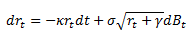
where κ is the continuous drift and σ is the continuous volatility.
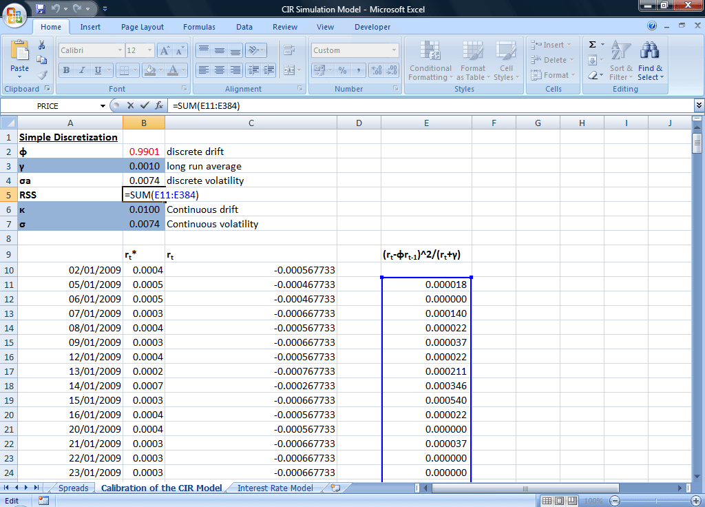
For the centered CIR model we need to determine a transformed short rate by subtracting the long run average (γ = AVERAGE (array of rates)) of the short rate from each rate observation (rt*), i.e. the transformed short rate rt is equal to rt*- γ.
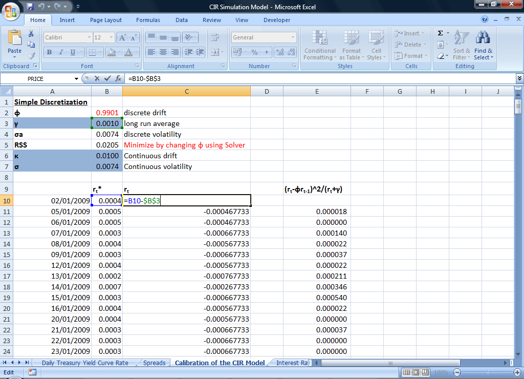
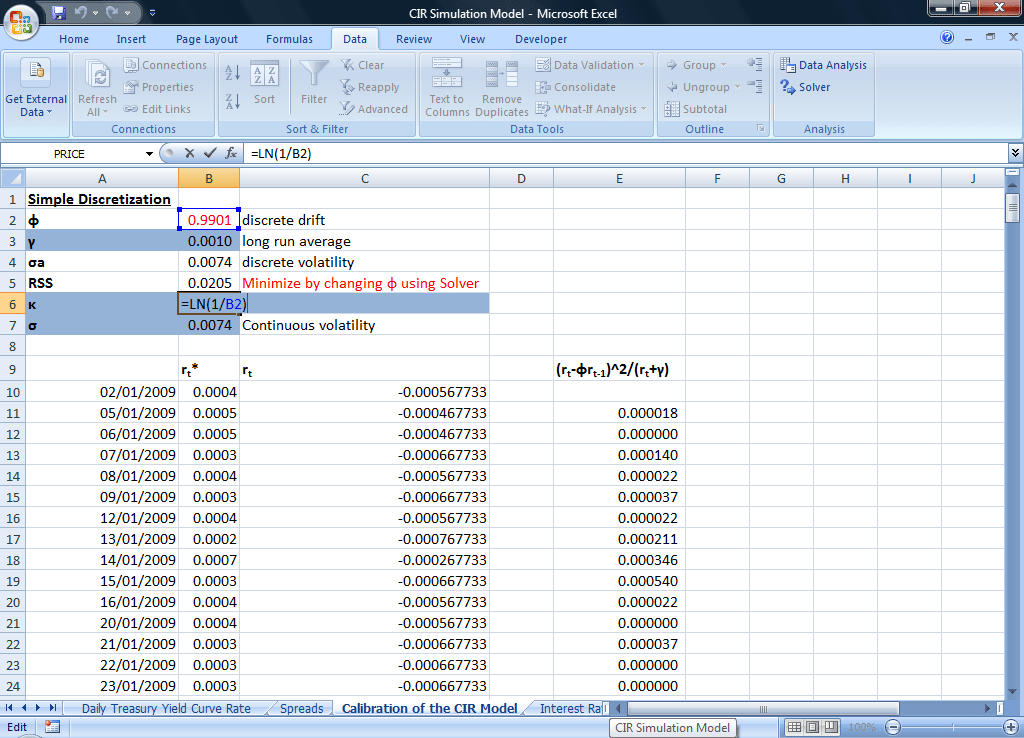
In our illustration, we have used the simple discretisation process to determine the parameters of the model. Under this process, the residual term is calculated at each data point as:

Phi , the discrete drift term, is first taken as an arbitrary number. The calibrated value, or least squares estimate for this term, will be determined after the sum of the residual terms (RSS) is minimized using the Solver function.
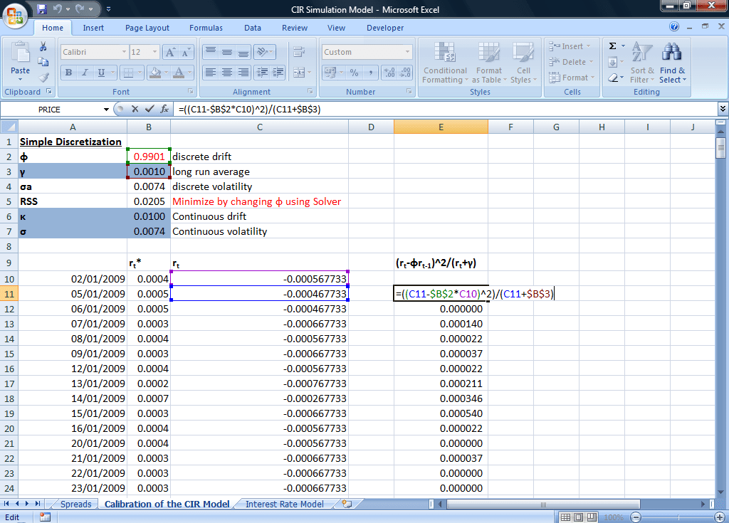
The RSS as mentioned above is the sum of the residual terms:
We next set up the solver function:
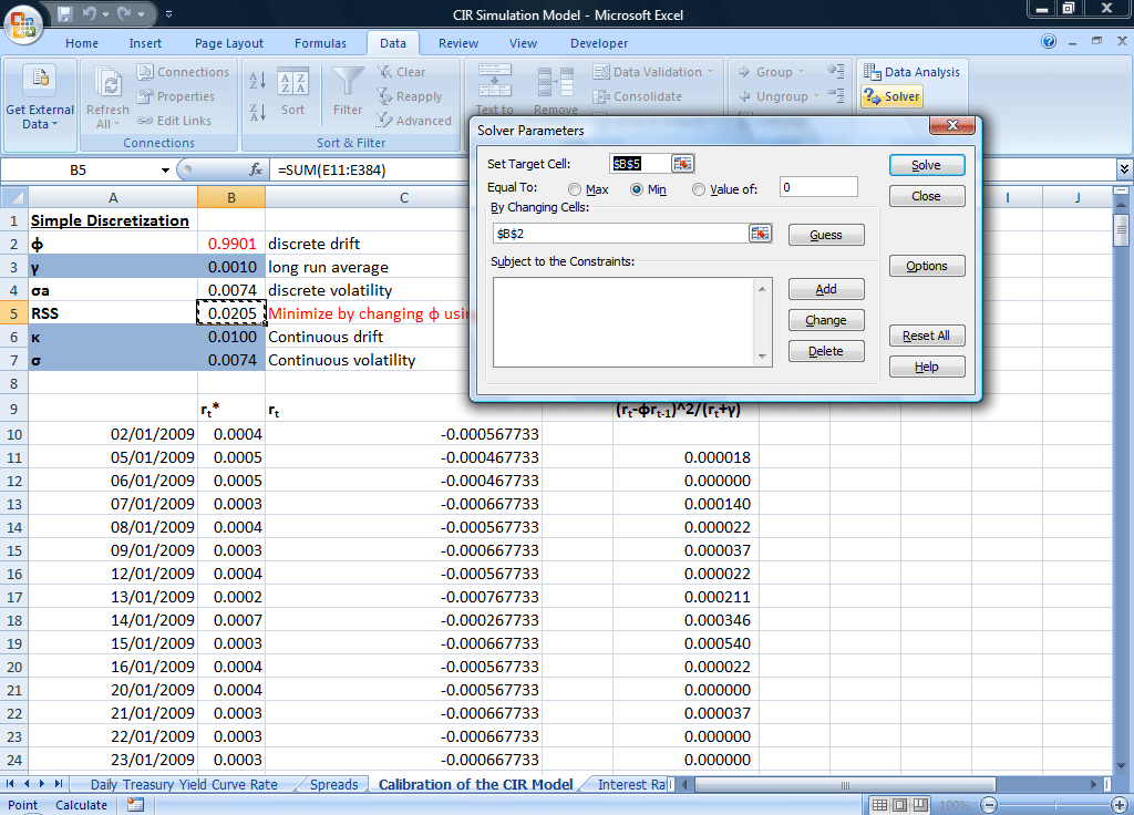
Go to the Data tab on the EXCEL worksheet and select Solver. Then
- Set Target Cell = the cell where residual terms are being summed, i.e. RSS (cell B5 in our illustration)
- Equal to: Min (because we are calibrating parameters by minimizing the sum of the residual terms)
- By Changing Cells = the cell for the value of the discrete drift term, i.e. Φ (cell B2 in our illustration)
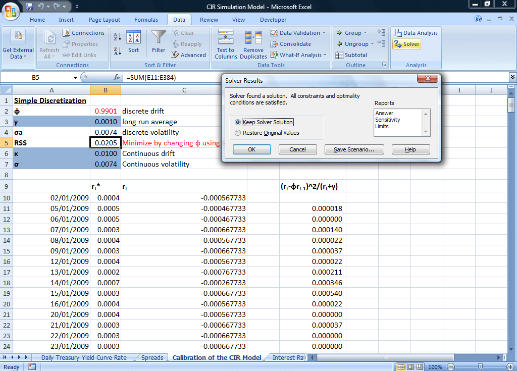
Run the Solver function by clicking on “Solve” to find an optimal solution:
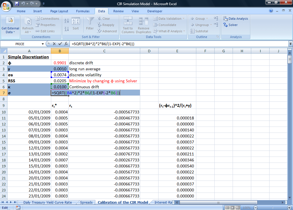
Calculating the parameters – discrete vol, continuous drift, continuous vol
The next stage of the calibration process is to use the results obtained after running Solver to calculate the:
- Discrete volatility parameter, σa = √(RSS/(N-1)), where N is the number of residual terms
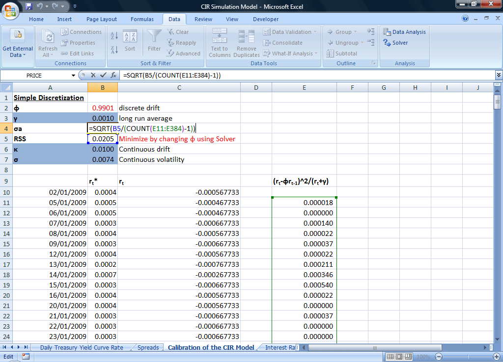
- Continuous drift, κ = -ln Φ = ln(1/ Φ)
- And continuous volatility, σ = √[(2κσa2)/(1-e-2κ)]
STEP 4: Simulate short rates
We use the calibrated and derived parameters together with the centered CIR model to simulate the short rate.
Recall the Centered CIR model is given as:
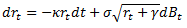
This may be restated for the actual short rate rt* as:
Δrt* = κ(γ-rt-1*)dt + σ√(rt-1*)dzt
Given that r0* = short rate as at 27-Jul-2010 = 0.16%
dt =1/360 (i.e. a daily time step assuming a 360 day year). Read the following post “CIR Interest Rate Model – Appropriate Time Step” to determine the correct time step to use in the interest rate model.
dz = NORMSINV(RAND())*√dt (normally scaled random number times the square root of the time step)
For ∆r1* = κ(γ-r0*)dt + σ√(r0*)dz1 =0.0019%
And Projected r1* = r0* + ∆r1*= 0.16%+0.0019% =0.1619%
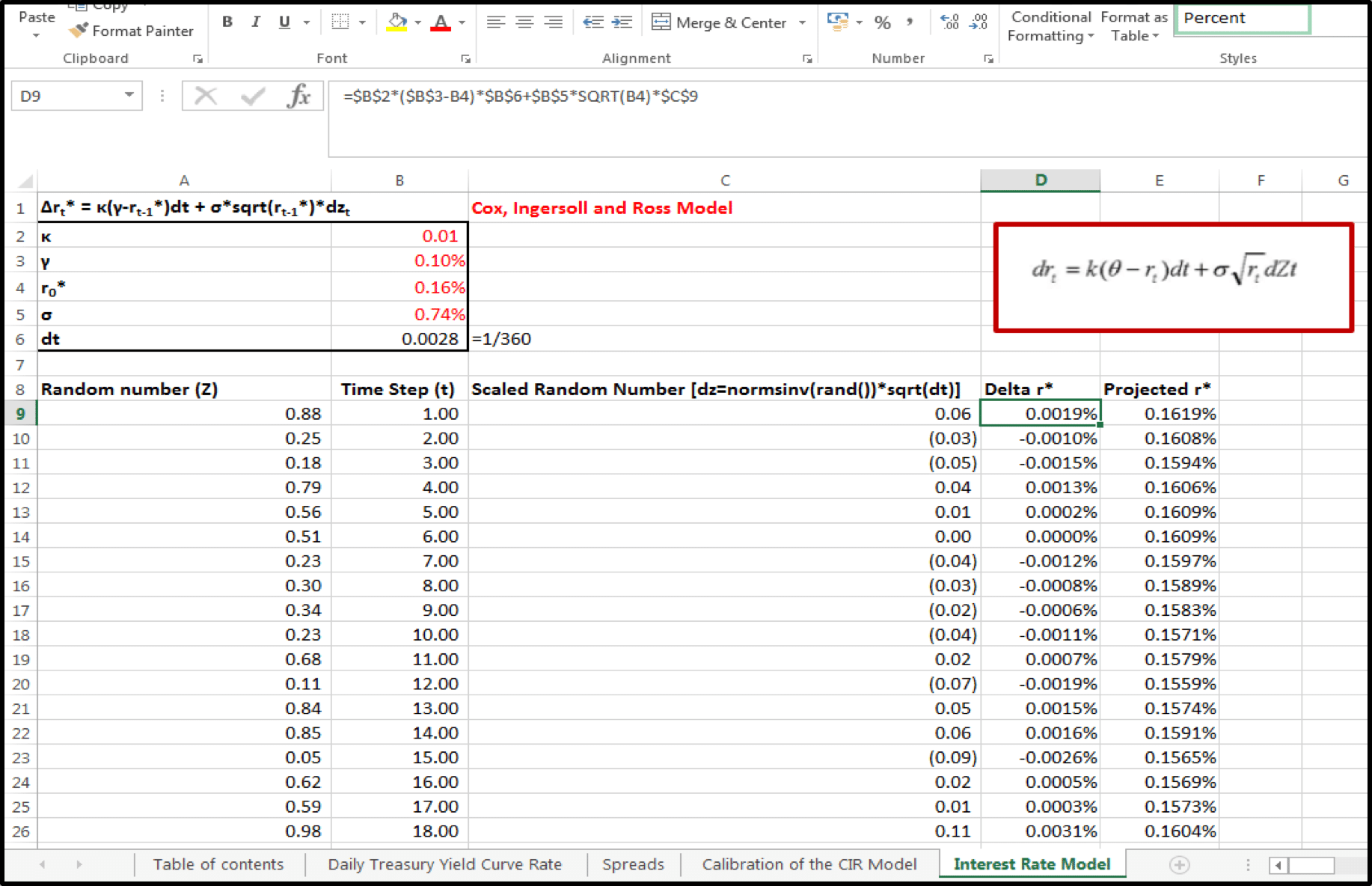
For r17* = r16* + ∆r17* = 0.1569% + 0.0003% =0.1573%.
Note: Clicking F9 will cause the series of simulated rates to change.
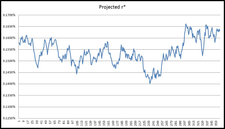
Below is a depiction of one simulation run of the projected short rates over a 360 day period:
STEP 5: Determining long term rates
We had briefly talked about how to model longer term rates once we have projected the short rates in the following post:
In particular, we had mentioned two specific ways of doing this by either assuming that:
1) Long term rates change by the same proportion as short term rates, or
2) Current spreads between the short rate and longer term rate are representative of future spreads
In the first case, we calculate the projected long term rate at time step t as:
Long term ratet =rt/r0*long term rate0
e.g. 2-month rate = 0.18%/0.16% * 0.155% = 0.17438%
The following is a representation of the term structure of interest rates over the next five time steps using this proportional method to determine long term rates:
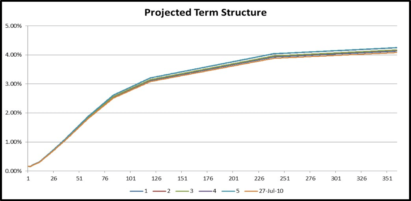
“27-Jul-2010” is the term structure today, “1” is the simulated term structure one month later, “2” is the simulated term structure two months down the line, and so on…
In the second instance, we calculate the projected long term rate at time step t as:
Long term ratet =rt + (long term rate0-r0)
e.g. 2-month rate = 0.18% + (-0.005%) =0.175%
The graph for the simulated term structures using a constant spread approach is given below:
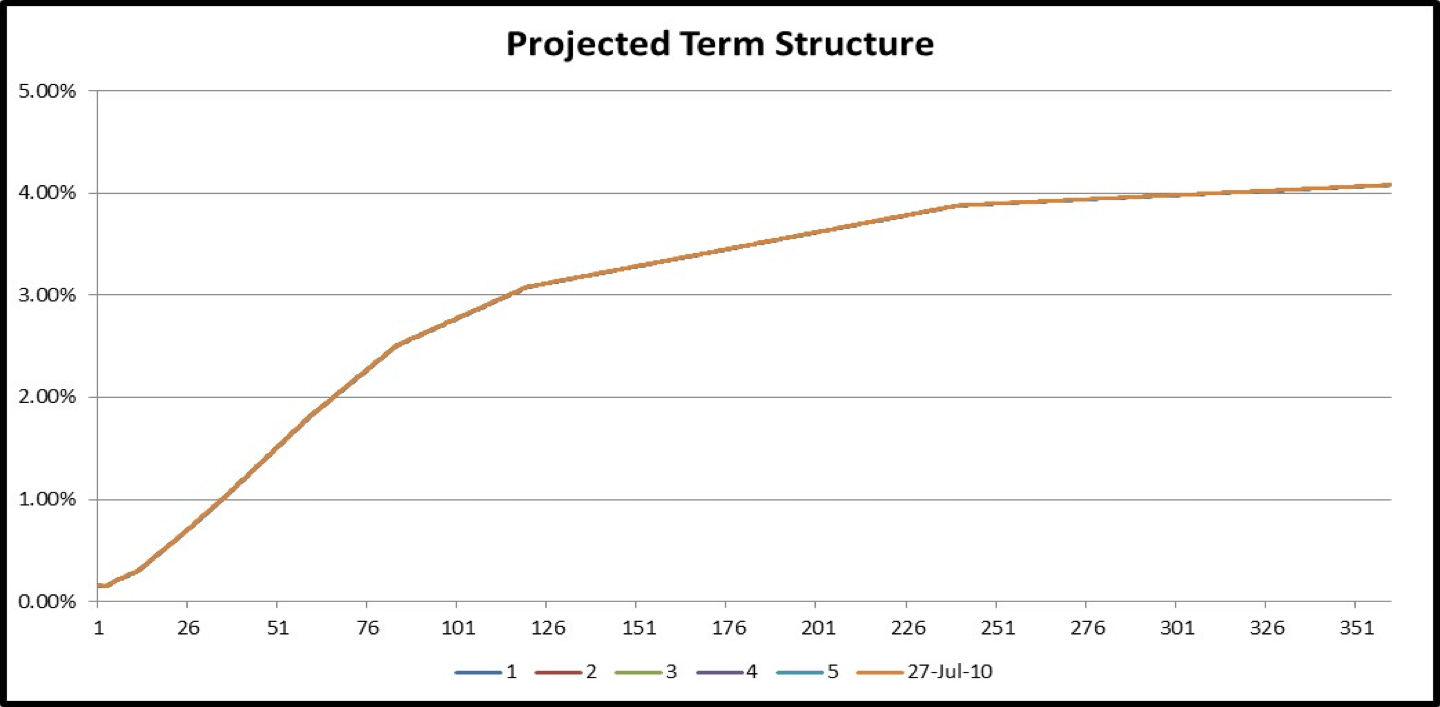
Note that in both cases the long term rates are perfectly correlated with the short rates.

Comments are closed.