The conventional way for pricing interest rate swaps (IRS) [with quarterly settlements] is to discount the future cash flows of the swap with discount factors calculated from the [3-month] London Interbank Offer Rate (LIBOR). However, following the Global Financial Crisis of 2007-2009, when spreads between the LIBOR and Overnight Indexed Swap (OIS) rates widened, there has been a change from using LIBOR discounting to OIS discounting for OIS swap pricing models to MTM interest rate swaps.
The following presentation is a summary of the paper “Valuing Interest Rate Swaps Using OIS Discounting” by Donald J. Smith (July 2012- Boston University School of Management Research Paper Series). The paper illustrates how swaps are valued using, in turn, LIBOR and Overnight Indexed Swap rates.
1. What is an Overnight Indexed Swap?
An overnight indexed swap is a derivative contract on the total return of a reference rate that is compounded daily over a specific time period. In the US, this reference rate is the effective federal funds rate, i.e. the weighted average of brokered trades between banks for overnight ownership of bank reserves. This rate is calculated and released daily by the Federal Reserve in its H.15 report.
2. Reasons for Switching from LIBOR to OIS Discounting
The major reason for switching from using LIBOR to the OIS as a term structure for pricing interest rate swaps is that OIS discounting better reflects the counterparty credit risk in a collateralized interest rate swap.
In recent years, the use of collateralization in the interest rate swap market has become standard practice in order to mitigate counterparty credit risk. During the 1990’s, after the introduction of the Credit Support Annex (CSA) in the standard International Swap and Derivatives Association (ISDA) master agreement, it became a norm to post collateral in the form of market securities or cash. Bilateral CSAs with zero thresholds, require the counterparty with the credit risk (negative swap value) in the transaction to post collateral. Due to these developments/ requirements, the credit risk on swaps has reduced significantly. As a consequence, the discount factors used to price these swaps need to be based on (near) risk-free interest rates. Treasury yields are not a feasible option for discounting swap cash flows because they tend to be too low for this purpose due to being highly liquid and tax free and generally more volatile.
Typically you would look to use discount factors based on the yields of securities which have the same liquidity, tax status, and volatility as the interest rate swaps with the addition conditional of having credit risk profile that approaches zero. Before 2007, traders and analysts considered the LIBOR to be a good proxy to produce the risk-free yield curve required for pricing interest rate swaps. In recent years, the LIBOR-OIS spread has persistently widened, particularly after August 2007. While LIBOR discounting may still be feasible for pricing uncollateralized IRS, dealers now prefer to use OIS discounting to value collateralized interest rate swaps because the OIS curve does not factor in the bank credit and liquidity risk that is inherently priced in LIBOR. Thus, OIS rates can now be seen as (near) risk-free interest rates with credit risk approaching zero.
3. Pricing Interest Rate Swaps Using LIBOR
We will first look at the example provided in the paper referenced above – a 2-year interest rate swap with USD 100 million notional principal, 5.26% fixed vs 3-month LIBOR that is settled on a quarterly frequency. The comparable fixed rate on at at-market swap is 3.40%. The day count convention assumed is Actual/360. In general, the methodology entails the following four steps:
- Step 1: Obtain the term structure. For LIBOR discounting this means cash market rates (for LIBOR deposits) for the first twelve months and the at-market swap fixed rates for the remaining tenor. For OIS discounting this means the OIS fixed rates for the tenor.
- Step 2: Calculate the discount factors
- Step 3: Calculate the implied LIBOR forward rates
- Step 4: Value the IRS in either of two ways:
- Step 4a – As a combination of long and short positions of implicit fixed and floating rate bonds
- Step 4b – As a series of forward contracts on the reference rate (e.g. 3 Month LIBOR)
Each of these two methodologies under step 4 follows the process below:
- Determine the future cash flows
- Discount the cash flows to the valuation date
- Sum the discounted cash flows
Step 1 – Obtain the term structure
For the first twelve months, observations of LIBOR deposit rates are used. For a quarterly settled swap, LIBOR rates for each quarter will be obtained:
| Period | Number of days in the period | LIBOR deposits rates |
| 1 | 92 | 0.50% |
| 2 | 92 | 1.00% |
| 3 | 91 | 1.60% |
| 4 | 90 | 2.10% |
For periods beyond 12 months, observations of fixed rates on at-market (par) swaps will be used:
| Period | Number of days in the period | Swap fixed rates |
| 5 | 92 | 2.44% |
| 6 | 92 | 2.76% |
| 7 | 91 | 3.08% |
| 8 | 90 | 3.40% |
The complete term structure that will be used is as follows:
| Period | Number of days in the period | LIBOR deposits /Swap fixed rates |
| 1 | 92 | 0.50% |
| 2 | 92 | 1.00% |
| 3 | 91 | 1.60% |
| 4 | 90 | 2.10% |
| 5 | 92 | 2.44% |
| 6 | 92 | 2.76% |
| 7 | 91 | 3.08% |
| 8 | 90 | 3.40% |
Step 2 – Calculate discount factors
Within the first twelve months, the general formula for calculating the quarterly LIBOR discount factors is the following,
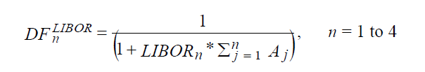
where
- DFnLIBOR = Discount factor for period n, discounting from end of period n to inception date.
- LIBORn = LIBOR deposit rate for period n
- Aj is the fraction of the year for the jth period. In the illustration, for period 2, ∑Aj = (92+92)/360 =184/360 days.
Using simple interest to determine interest cash flows, the above equation is a rearrangement of the equation to solve for the discount factor, which equates the par value of the bond at inception, i.e. USD 1 per unit to the present value of the principal and interest cash flows where the cash flows are discounted from the settlement date to the inception date.
For period 2, for example, this is:
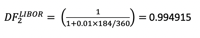
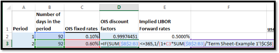
In EXCEL for period 2 this formula has been applied as follows:
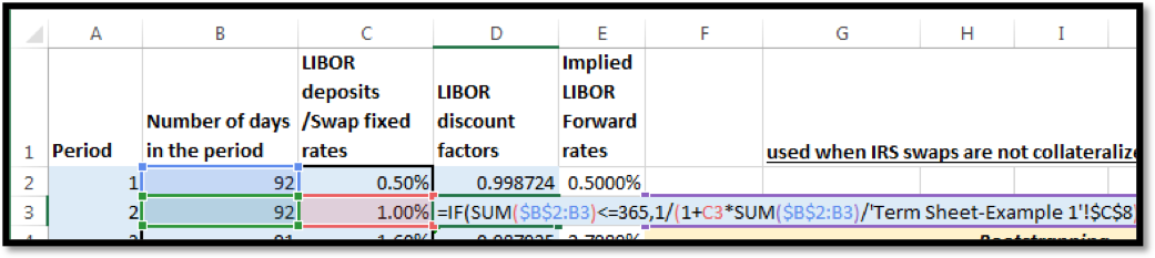
Where ‘Term Sheet – Example 1’!$C$8 in the formula above is 360
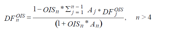
Beyond the first 12-month period, discount factors are calculated by bootstrapping fixed rates on at-market swaps. The at-par swap (per unit value of 1 at inception) is treated as a fixed rate, non-amortizing par value bond. The bond is stripped of its coupon and (non-amortizing) principal payments, and each cash flow is then discounted to inception from its settlement date separately as a zero coupon or bullet bond.
The general formula for bootstrapping LIBOR discount factors from at-market swap fixed rates (SFR’s) is:

where
- DFnLIBOR = Discount factor for period n, discounting from end of period n to inception date.
- SFRn = At-market swap fixed rate for period n
- Aj is the fraction of the year for the jth period. In the illustration, for period 5, A5 = 92/360.
The equation above is a rearrangement of the equation, to solve for the discount factor at period n, which equates the par value of the bond at inception (i.e. USD 1 per unit) to the present value of cash flows, where each individual cash flow is discounted from the date of its settlement to the date of inception.
For example at period 5 the at-par bond has the following cash flows. Coupon payments at a fixed rate of 2.44% for periods 1 -5 and principal payment of 1 at the end of period 5. Coupon payments at periods 1 to 4 will be discounted by the LIBOR discount factors determined earlier. The sum of these discounted payments is deducted from the par value of the bond to arrive at the discounted value of the final principal and interest payment at the end of period 5. Dividing this value with the undiscounted principal and interest cash flow for period 5 will result in the discount factor applicable from the period 5 settlement date to inception.
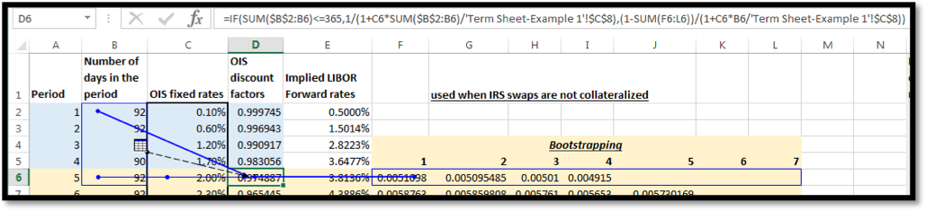
In EXCEL this formula is applied as follows for period 5:
First, we individually discount the coupon cash flows at periods 1-4
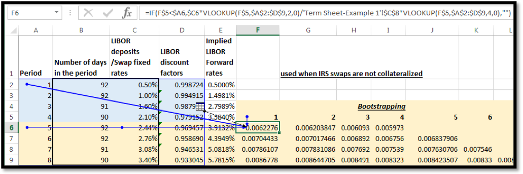
Where ‘Term Sheet – Example 1’!$C$8 in the formula above is 360
What we are doing in cell F6 in the screenshot above is multiplying the first coupon (@2.44%) with the number of days in the first period (92) dividing by 360 as per day count convention and then multiplying the result with the already derived LIBOR discount factor for period 1. We repeat this process for the cash flows at periods 2-4.
Then we subtract the sum of discounted cash flows from 1 and divide the resulting value with the coupon and principal cash flow of period 5 to arrive at the LIBOR discount rate for period 5, as follows (indicated in the second half of the EXCEL formula [boxed in red]:
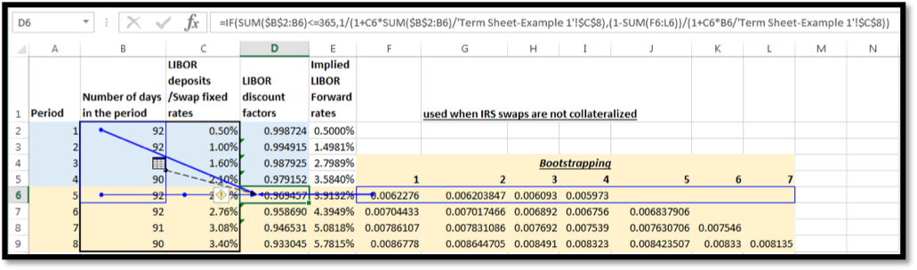
Where ‘Term Sheet – Example 1’!$C$8 in the formula above is 360.
Step 3 – Calculate implied LIBOR forward rates
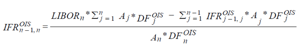
Another important term is that of the implied forward rate (IFR), which is also known as the projected forward rate for a 3-month LIBOR between n-1 and n periods. It is derived from successive discount factors and calculated using the following formula:
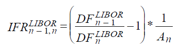
The implied LIBOR forward curve is useful in pricing options on swaps and non-standard interest rate swaps. An example of a non-standard interest rate swap is of a swap whose notional principal varies over its tenor.
In EXCEL the formula for IFR above is applied as follows:
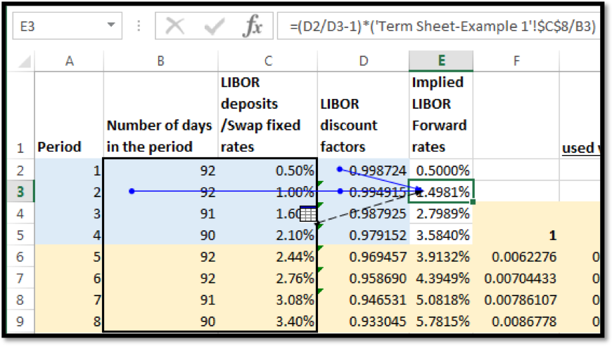
Where ‘Term Sheet – Example 1’!$C$8 in the formula above is 360
Note: For period 1, the implied forward rate is equal to the LIBOR deposit rate for that period, i.e. 0.50%.
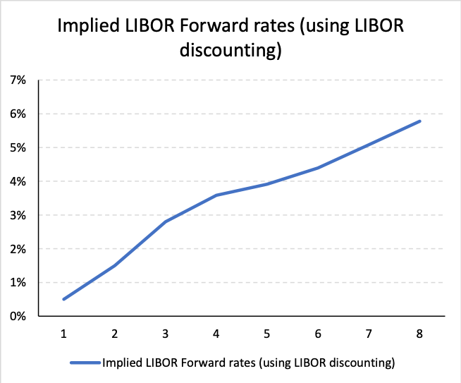
A graphical representation of the term structure of implied forward rates is depicted below:
Step 4a: Value the IRS as a combination of bonds
The value of the interest rate swap is determined by calculating the value of the two bonds implicit in the interest rate swap. First, the price of the Floating Rate Note (FRN) is calculated as follows:
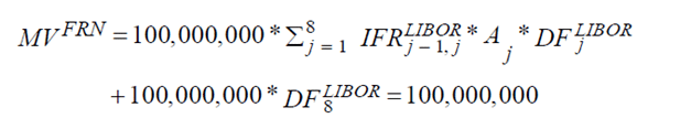
Then the price of the 5.26% fixed rate note is calculated as follows:
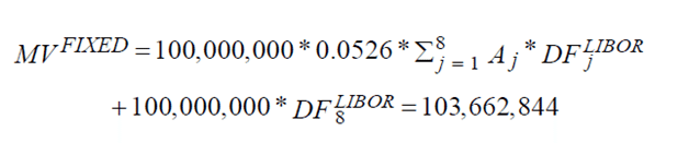
The difference in the price of these bonds is equal to the market value of the swap, which is as follows:

In EXCEL this may be accomplished in the following stages:
i. Determine the future cash flows
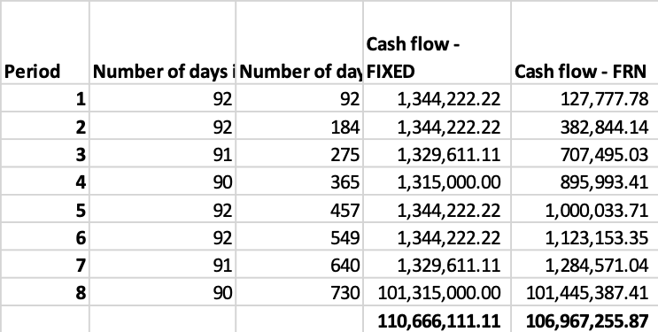
For the Fixed bond, this is the coupon payment at 5.26% (adjusted for the days in the period with respect to a 360 day year) times the notional amount for each of the eight periods and the principal (notional amount) at maturity at the end of period 8. For example, the cash flow at period 8 is:
100,000,000 x 0.0526 x 90/360 + 100,000,000 = USD 101,315,000.00
For the Floating rate bond, this is the coupon payment at the implied forward rate for the period (adjusted for the days in the period with respect to a 360 day year) times the notional amount for each of the eight periods and the principal (notional amount) at maturity at the end of period 8. For example, the cash flow at period 8 is:
100,000,000 x 0.057815 x 90/360 + 100,000,000 = USD 101,445,387.41
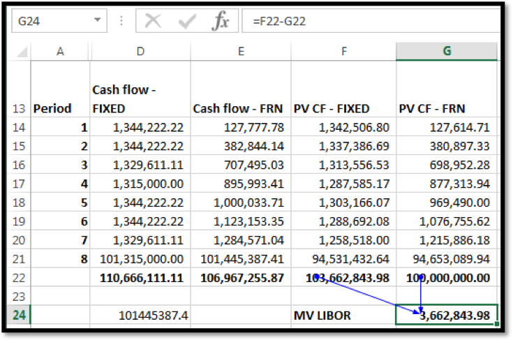
ii. Discount the cash flows to the valuation date
The cash flows are discounted using the calculated discount factor for the period. For period 8 both the fixed and the floating rate cash flows are discounted by 0.933045. The discounted cash flows for period 8 are:
- 101,315,000.00 * 0.933045 = USD 94,531,432.64 for the fixed rate bond, and
- 101,445,387.41 * 0.933045 = USD 94,653,089.94 for the floating rate bond
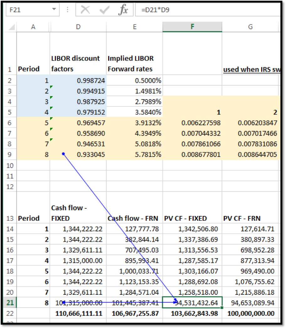
iii. Sum the discounted cash flows
The sum of the discounted cash flows gives the price of the Fixed and Floating Rate bonds respectively. The difference between the prices gives the value of the IRS:
Price of Fixed Bond = USD 103,662,843.98
Price of Floating Rate Bond = USD 100,000,000.00
Price of IRS = Price of Fixed Bond – Price of Floating Rate Bond = USD 3,662,843.98
Step 4b: Value the IRS as a series of forward contracts on the reference rate
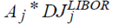
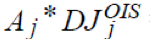
The net cash flow for the receiver of the fixed rate leg of the swap is the Notional x (fixed rate minus at-market swap rate for the given tenor) at each settlement date. In our example, the fixed rate is 5.26% while the at-market swap for the 2-year IRS is 3.40%. We adjust each payment for the days in the period and discount the net cash flow using the LIBOR discount factor. As the cash flow is based on fixed rates, the period adjusted discount factors can be summed before multiplying by Notional x (fixed rate minus at-market swap rate for the given tenor).
In the paper the formula is given as:
In EXCEL, we determine for each period first:

Where ‘Term Sheet – Example 1’!$C$8 in the formula above is 360.
And then sum these values across all the periods:
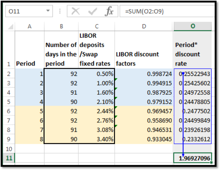
Next we multiply this sum with the notional times the difference between the fixed rate & at-market rate to determine the value of the IRS: 100,000,000 x (0.0526-0.034) x 1.96927096 = USD 3,662,843.98
To reiterate, the main assumption made in the above calculations is that the LIBOR is an effective proxy for the near risk free yield curve needed for pricing a collateralized swap. However, based on the following developments this is no longer true:
- Collateralization is now the norm in the market
- The LIBOR-OIS spread is significant and cannot be ignored.
Thus, due to these two conditions, it has become necessary to use OIS discounting to price interest rate swaps.
4. Pricing Interest Rate Swaps using OIS swap pricing / OIS discounting
The same 2-year interest rate swap on a USD 100 million notional amount used in illustrating LIBOR discounting above is assumed. The pricing of the IRS using OIS discounting follows almost the same four step process mentioned above with two main differences:
- Instead of LIBOR deposits and swap fixed rates being used OIS rates are used.
- A new implied LIBOR forward rate formula is calculated so that the value of the IRS determined under both valuation methods mentioned in Step 4a & Step 4b will be consistent and give the same results.
Step 1 – Obtain the term structure
The complete term structure that will be used is as follows:
| Period | Number of days in the period | OIS fixed rates |
| 1 | 92 | 0.10% |
| 2 | 92 | 0.60% |
| 3 | 91 | 1.20% |
| 4 | 90 | 1.70% |
| 5 | 92 | 2.00% |
| 6 | 92 | 2.30% |
| 7 | 91 | 2.60% |
| 8 | 90 | 2.90% |
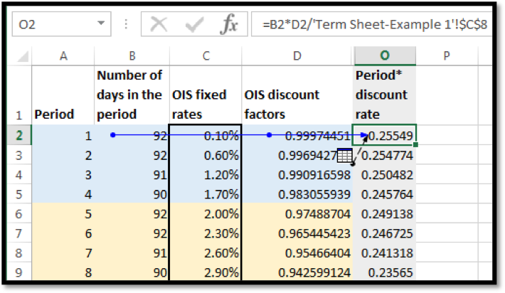
Step 2 – Calculate discount factors
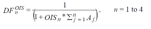
The process is similar to determining LIBOR discount factors. For the periods within 12 months the following formula is used:
In EXCEL for period 2, the formula is applied as follows:
You can see that the formula used is the same as in the EXCEL worksheet for LIBOR discount factors (with the exception of the rate inputs in column C).
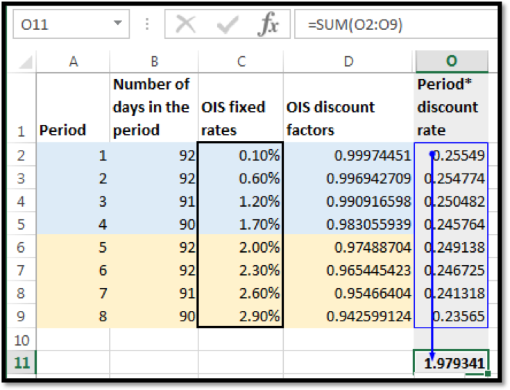
For periods beyond twelve months the following general formula for bootstrapping the OIS discount factors is used:
Again the formula in EXCEL is the same as that used earlier for the LIBOR discount factors:
Where ‘Term Sheet – Example 1’!$C$8 in the formula above is 360.
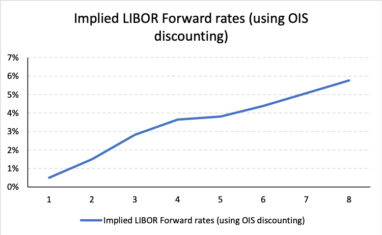
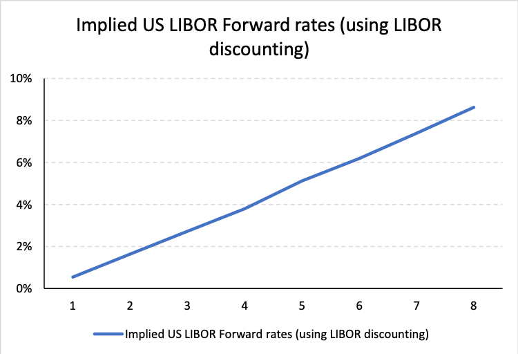
Step 3 – Calculate implied LIBOR forward rates
In order to find the value of the implicit FRN note for Step 4a below it is essential that a new LIBOR forward curve is generated. This is important because OIS discount rates are now being used to price the swap. Therefore a forward curve which prices LIBOR deposits and at-market LIBOR swaps with OIS discount factors is needed.
For the money market segment of the swap curve, i.e. from n=1 to n=4, the following formula is used to calculate the implied forward rates:
For n>4, the at-market LIBOR swap fixed rates are used instead of the LIBOR deposit rate:
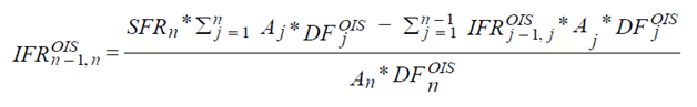
In EXCEL the formula is applied as follows for all periods, except period 1:
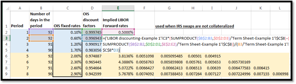
Where ‘Term Sheet – Example 1’!$C$8 in the formula above is 360
‘LIBOR discount-Example 1’!C3 is the LIBOR deposit rate for period 2. [Note: For periods 1-4, LIBOR deposit rates are referenced while for periods 5-8 the swap fixed rates are referenced].
Note: For period 1, the implied forward rate is equal to the LIBOR deposit rate for that period, i.e. 0.50%.
The implied LIBOR forward rate term structure is graphed below:
Step 4a: Value the IRS as a combination of bonds
The price of the swap is determined by finding out the market values of the implicit fixed rate and the floating rate bonds. The same three step methodology and formulas in EXCEL described above for LIBOR discounting is used to determine the price of each bond.
i. Determine the future cash flows
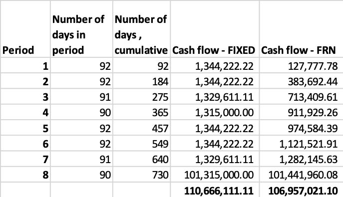
ii. Discount the cash flows to the valuation date
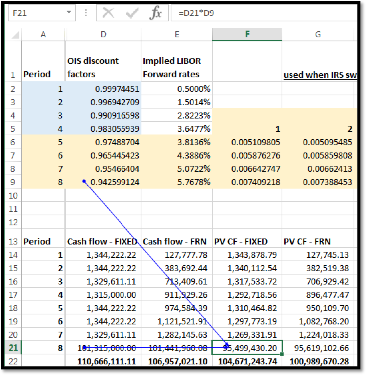
iii. Sum the discounted cash flows
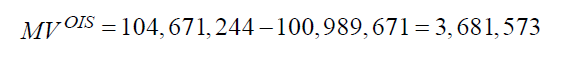
The sum of the discounted cash flows gives the price of the Fixed and Floating Rate bonds respectively. The difference in prices gives the value of the IRS:
Price of Fixed Bond = USD 104,671,243.74
Price of Floating Rate Bond = USD 100,989,670.28
Price of IRS = Price of Fixed Bond – Price of Floating Rate Bond = USD 3,681,573.46
Step 4b: Value the IRS as a series of forward contracts on the reference rate
The net cash flow for the receiver of the fixed rate leg of the swap is the Notional x (fixed rate minus at-market swap rate for the given tenor). In our example, the fixed rate is 5.26% while the at-market swap for the 2-year IRS is 3.40%. We adjust each payment for the days in the period and discount using the LIBOR discount factor.
In the paper the formula is given as:
In EXCEL we determine for each period first:
Where ‘Term Sheet – Example 1’!$C$8 in the formula above is 360.
And then sum these values across all the periods:
We then multiply this sum with the notional times the difference between the fixed rate & at-market rate to determine the value of the IRS: 100,000,000 x (0.0526-0.034) x 1.979341 = USD 3,681,573.46.
5. OIS Discounting vs LIBOR – Conclusion
The market value of the swap using OIS discount rates is higher at USD 3,681,573, compared with the market value of the swap priced at USD 3,662,844 using LIBOR discount rates.
This higher price is a reflection of the reduced credit risk on the collateralized interest rate swap as compared to the uncollateralized counterpart. OIS discounting is a more accurate way of stating the price of a collateralized interest rate swap given that the LIBOR term structure can no longer be considered a risk free yield curve proxy.
6. OIS vs LIBOR Example Two
While the first example is the original reproduction from Donald Smith’s paper, we now present a second illustrated example where we work with two IRS.
The derivatives are 2-year interest rate swaps with USD 100,000 and EUR 100,000 notional principals respectively, 5.5% fixed vs 3-month USD LIBOR/ EURIBOR settled quarterly. The comparable at-market fixed rates are equal to the last quarter swap fixed rates. We assume a 90/360 day count convention for each.
LIBOR discounting
The observed US LIBOR deposit/swap fixed rates and EURIBOR deposit/ swap fixed rates are as follows:
| Period | US LIBOR deposits /Swap fixed rates | EURIBOR deposits /Swap fixed rates |
| 1 | 0.541% | 0.630% |
| 2 | 1.089% | 1.268% |
| 3 | 1.638% | 1.908% |
| 4 | 2.189% | 2.552% |
| 5 | 2.744% | 3.200% |
| 6 | 3.302% | 3.852% |
| 7 | 3.863% | 4.509% |
| 8 | 4.427% | 5.169% |
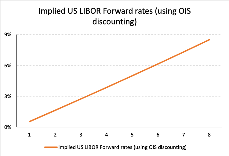
Under LIBOR discounting the USD LIBOR discount rates & implied USD LIBOR forward rates workout to:
| Period | Number of days in the period | US LIBOR deposits /Swap fixed rates | US LIBOR discount factors | Implied US LIBOR Forward rates |
| 1 | 90 | 0.541% | 0.9986493 | 0.5410% |
| 2 | 90 | 1.089% | 0.9945845 | 1.6348% |
| 3 | 90 | 1.638% | 0.9878641 | 2.7212% |
| 4 | 90 | 2.189% | 0.9785789 | 3.7954% |
| 5 | 90 | 2.744% | 0.9662084 | 5.1212% |
| 6 | 90 | 3.302% | 0.9514823 | 6.1908% |
| 7 | 90 | 3.863% | 0.9342171 | 7.3924% |
| 8 | 90 | 4.427% | 0.9144917 | 8.6280% |
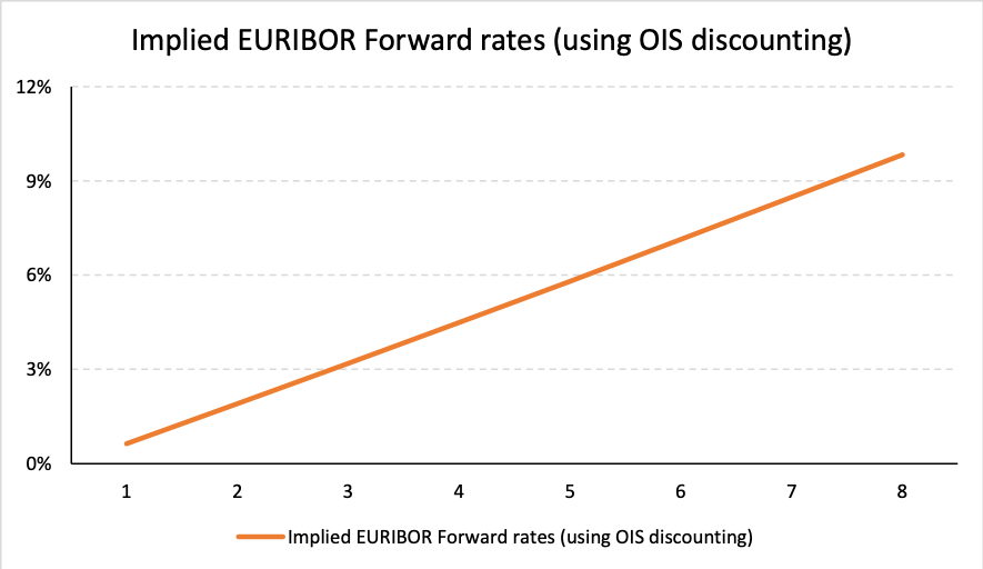
While the EURIBOR discount rates & implied EURIBOR forward rates are determined as:
| Period | Number of days in the period | EURIBOR deposits /Swap fixed rates | EURIBOR discount factors | Implied EURIBOR Forward rates |
| 1 | 90 | 0.630% | 0.9984275 | 0.6300% |
| 2 | 90 | 1.268% | 0.9936999 | 1.9030% |
| 3 | 90 | 1.908% | 0.9858919 | 3.1679% |
| 4 | 90 | 2.552% | 0.9751151 | 4.4207% |
| 5 | 90 | 3.200% | 0.9606894 | 6.0064% |
| 6 | 90 | 3.852% | 0.9435931 | 7.2473% |
| 7 | 90 | 4.509% | 0.9235614 | 8.6758% |
| 8 | 90 | 5.169% | 0.9007331 | 10.1377% |
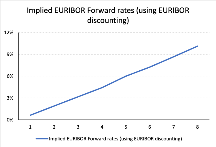
The two implied forward curves are also plotted graphically below:
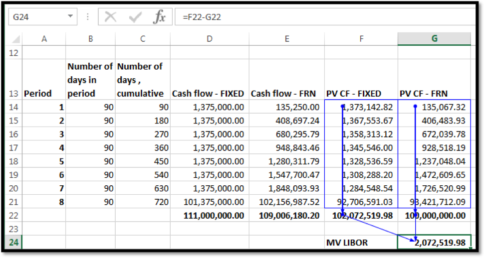
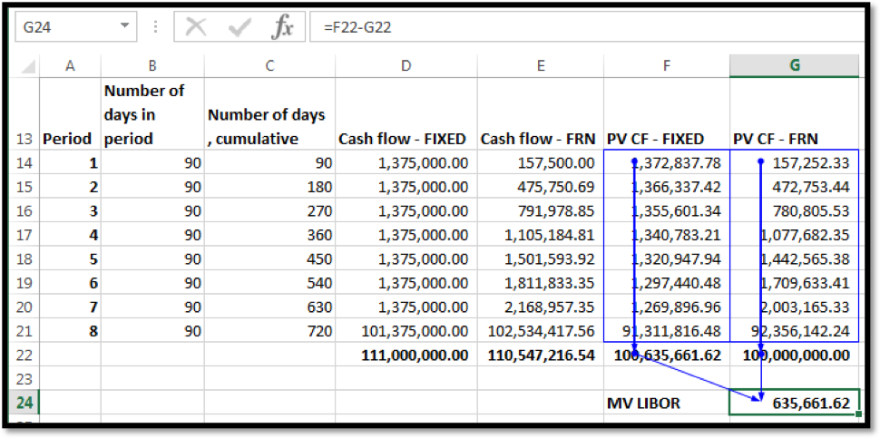
We use the methodology at Step 4a above to determine the value of the IRS, i.e. the difference in the value of two implicit bonds.
For the USD denominated IRS the valuation model is as follows:
For the EUR denominated IRS the price is determined as follows:
OIS Discounting
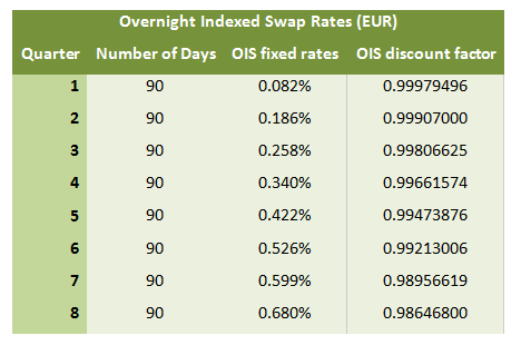
The same instruments are now valued using OIS rates. The observed OIS fixed rates are as follows:
| Period | OIS fixed rates (USD) | OIS fixed rates (EUR) |
| 1 | 0.270% | 0.082% |
| 2 | 0.542% | 0.186% |
| 3 | 0.814% | 0.258% |
| 4 | 1.087% | 0.340% |
| 5 | 1.361% | 0.422% |
| 6 | 1.635% | 0.526% |
| 7 | 1.911% | 0.599% |
| 8 | 2.186% | 0.680% |
Under OIS discounting the OIS discount rates (USD) & implied USD LIBOR forward rates workout to:
| Period | Number of days in the period | OIS fixed rates (USD) | OIS discount factors | Implied US LIBOR Forward rates |
| 1 | 90 | 0.270% | 0.99932546 | 0.5410% |
| 2 | 90 | 0.542% | 0.99729732 | 1.6381% |
| 3 | 90 | 0.814% | 0.99393204 | 2.7408% |
| 4 | 90 | 1.087% | 0.98924689 | 3.8547% |
| 5 | 90 | 1.361% | 0.98311368 | 4.9907% |
| 6 | 90 | 1.635% | 0.9757258 | 6.1402% |
| 7 | 90 | 1.911% | 0.96700826 | 7.3082% |
| 8 | 90 | 2.186% | 0.95703045 | 8.4967% |
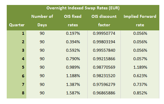
While the OIS discount rates (USD) & implied EURIBOR forward rates are determined as:
| Period | Number of days in the period | OIS fixed rates (EUR) | OIS discount factors | Implied EURIBOR Forward rates |
| 1 | 90 | 0.082% | 0.999795042 | 0.6300% |
| 2 | 90 | 0.186% | 0.999070864 | 1.9065% |
| 3 | 90 | 0.258% | 0.998068737 | 3.1897% |
| 4 | 90 | 0.340% | 0.996611521 | 4.4886% |
| 5 | 90 | 0.422% | 0.994737361 | 5.8015% |
| 6 | 90 | 0.526% | 0.992135749 | 7.1301% |
| 7 | 90 | 0.599% | 0.989562452 | 8.4796% |
| 8 | 90 | 0.680% | 0.986474025 | 9.8323% |
The implied forward curve plots are as follows:
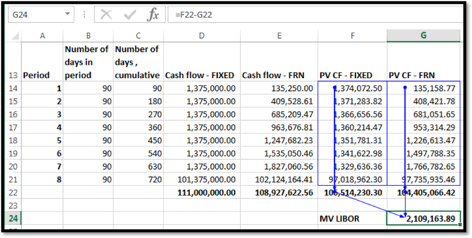
We use the methodology at Step 4a above to determine the value of the IRS, i.e. the difference in the value of two implicit bonds.
For the USD denominated IRS the valuation model is as follows:
For the EUR denominated IRS the price is determined as follows:
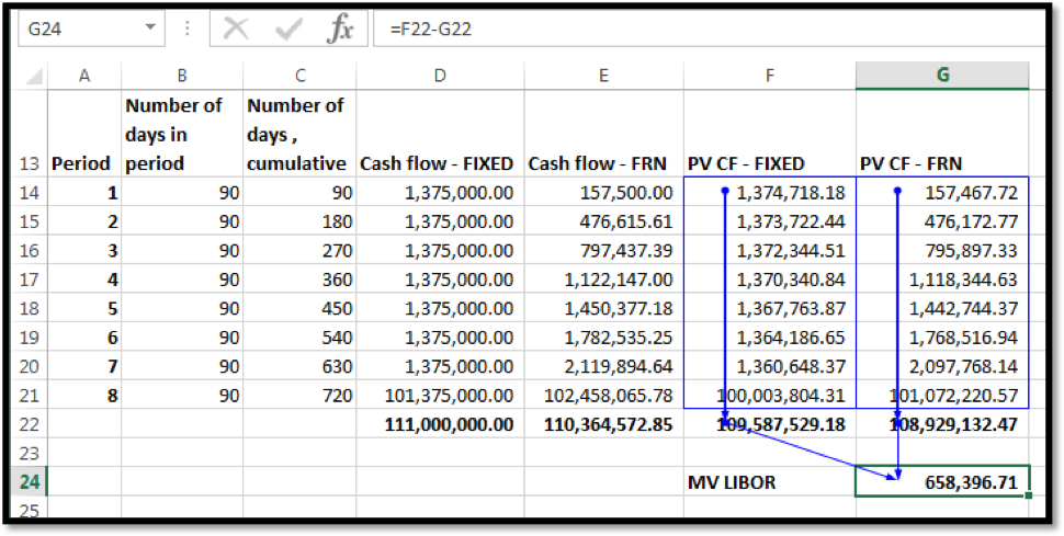
A side by side comparison of the results from the two approaches are given in the table below:
| LIBOR discounting | OIS discounting | |||
| USD | EUR | USD | EUR | |
| MV Fixed | 102,072,519.98 | 100,635,661.62 | 106,514,230.30 | 109,587,529.18 |
| MV Floating | 100,000,000.00 | 100,000,000.00 | 104,405,066.42 | 108,929,132.47 |
| MV of IRS | 2,072,519.98 | 635,661.62 | 2,109,163.89 | 658,396.71 |
As expected the values of the IRS are higher when swaps are priced using OIS swap pricing / OIS discounting.