When it comes to counterparty credit risk there are two credit exposure calculation methods that we frequently see in term sheets and internal risk reporting. Pre Settlement Risk Exposure (PSR or PSRE) and Potential Future Exposure (PFE). In this post, we present an overview of PFE calculations fora simple IRS.
PSR is a “static” measure based on a Value at Risk (VaR) estimate of worst case loss that would occur on a given transaction with a given counterparty at a given point in time. PSR is considered static because it looks at exposure only at a point in time irrespective of the life of the transaction. While PFE takes a forward looking approach to track how the transaction behaves over its life and the impact of that behavior on counterparty credit risk. For multi leg transactions such as interest rate swaps and cross currency swaps it is common to use both PSR and PFE to allocate credit risk limits. Both tools utilize a value at risk based model to forecast worst case market shocks but differ in how that shock impacts credit limit utilization.
The example below is based on a simple non amortizing interest rate swap. However, it can very easily be extended to profit rate swaps, options and other multi-leg transactions.

The transaction – An Interest Rate Swap
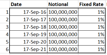
We use a simple non amortizing Interest Rate Swap for illustrating the PFE calculation model. Our interest rate swap is a 6 leg annual payment receive fixed swap. This means that the swap will pay a fixed rate once a year on a settlement date for the next six years. In return we, the owners of the swap will pay a floating rate on each settlement date. If interest rates decline from their current levels, our swap will increase in value. If interest rates rise, our swap will decrease in value. The date the swap is purchased is 15th September with net settlement happening on 17th September every year for the next six years. While we still have to agree on the fixed rate the expectation is that it will be set in a range between 1% and 3.5%.
The notional amount on the swap is USD 100,000,000.
Methodology for calculating Potential Future Exposure
We will need the following items to complete our PFE calculation exercise.
1) A valuation model for our interest rate swap.
2) An interest rate simulator or rates generator for predicting future interest rates.
3) An implied forward interest rate calculator.
For each interest rate swap in our portfolio we would need to:
- Identify points of interest (settlement dates or legs).
- Identify net exposure at points of interest.
- At each point estimate worst case market shocks for a given confidence level (include both normal and stressed conditions).
- Mark to market the transaction at points of interest.
- Plot positive MTM exposure at points of interest.
- Pick and plot peak exposure across points of interest.
The drivers – Forward Rates – Current and implied forward rates
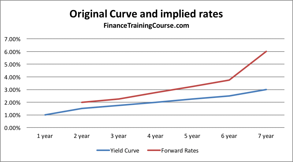
Current and implied future interest rates drives the value of our swap. To understand how to bootstrap implied forward rates from a yield curve please see the step by step calculation guide in the implied forward rate case study. The case study describes how to bootstrap rates and use them for marking to market interest rate swaps.
For the purpose of our PFE case study, we use the following yield curve and implied rates.
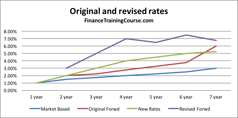
For our analysis, we use a simple shift in rates to generate our new yield curve. For a detailed review of multiple interest rate simulation approaches please see the interest rate simulation crash course.
Potential Future Exposure Calculation – Baseline
Now that we have our models and our rates together we are ready to estimate potential future exposure on our transaction.
We first estimate the value of the swap for both counterparties, the customer and the bank at time zero. To keep our calculations simple we ignore the impact of discounting (time value of money) in our valuation model . We just do a simple addition of cash flows for both the fixed rate receiver and the floating rate receiver.
Also, this set of calculations is done using the original yield curve and implied forward rates at time zero. It doesn’t include the impact of changes in interest rates, yield curves or implied forward rates.
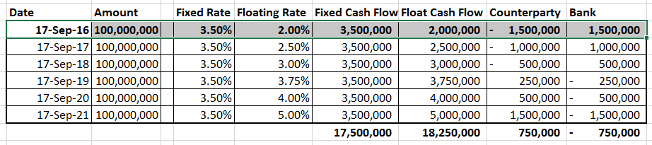
Time Zero – 18 September 2015
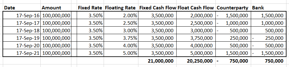
At time zero the mark to market valuation of the swap is USD -750,000 for the counterparty and USD 750,000 in favor of the bank.
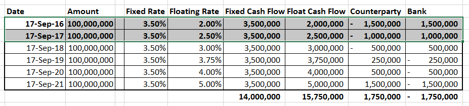
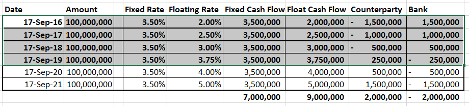
Time One – 18 September 2016
At time one the mark to market valuation of the swap is USD 750,000 for the counterparty and USD -750,000 in favor of the bank. The change happens because the first leg (highlighted) has been settled and is no longer included in future cash flows.
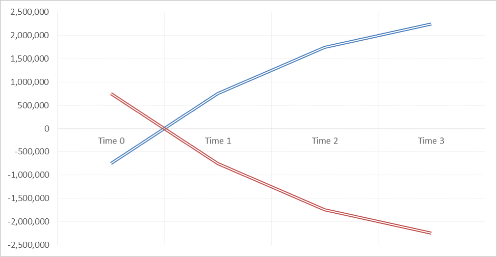
The plot of the two MTM’s at Time zero and Time one looks like the image below.
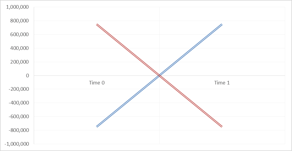
You can clearly see the flip in MTM from one leg to the next. We now repeat this process for the life of the transaction or the next four legs.
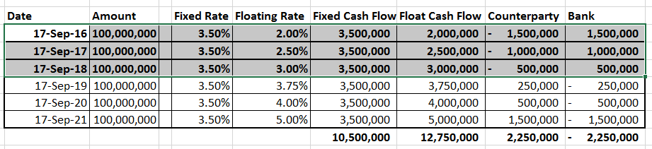
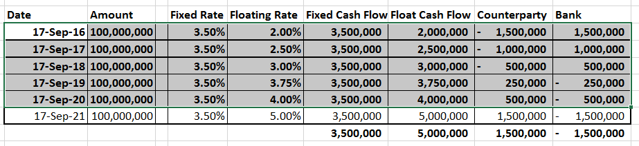
Time Two – 18 September 2017 – Post settlement of the first two legs
Time Three – 18 September 2018 – Post settlement of the first three legs
You should now be able to see a clear trend emerge from this data.
Time Four – 18 September 2019 – Post settlement of the first four legs
Time Five – 18 September 2020 – Post settlement of the first five legs
Putting it all together we get the trend for the exposure across the life of the transaction at current rates. Within the table below you can see both sides of the transaction. The counterparty (which is us) as well as the bank (the seller of the swap).
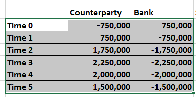
For the rates used and the swap structure in question, it appears that after the first leg, it will be the counterparty that will be exposed to the bank, rather than the other way around. While the counterparty may be in the money using the initial term structure that can quickly when the interest rate environment changes.
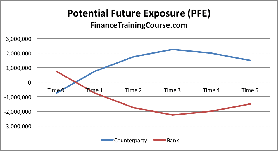
The graph above represents one possible future where we trace the exposure of the counterparties across the life of the swap.
Here is another path for the same transaction, calculated, plotted and tracked in a similar fashion, but for a different yield curve.
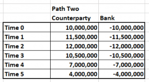
Compared to the first path this future takes a very different trajectory as well as a significantly larger peak exposure on year three.
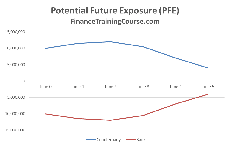
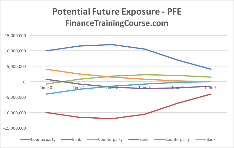
The PFE process essentially requires the ability to generate such paths, tabulate results using MTM valuations for a transaction on the path and then compiling peak exposures across all paths across the life of the transaction.
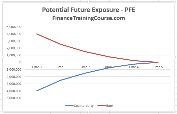
If we take this concept forward using a short sample of three paths, here is what our world would look like with the third and final path.
Summary of results for the three paths
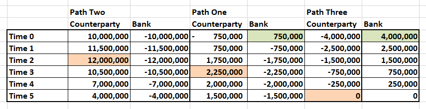
Compiling the three paths together in the table below we see that from the point of view of the counterparty (us) our primary exposure to the bank ranges between zero (Path three) to USD 12 million (Path two). This is our PFE estimate using our three paths sample world. From the bank’s point of view, their PFE estimate against us is USD 4 million (Path three). In % of notional terms, our PFE estimate is 12% of notional where the bank is our counterparty. While the bank’s PFE estimate on the same transaction is 4% of notional exposure.
While the three path approach is only illustrative, an actual PFE calculation exercise will follow a similar approach. However, rather than stopping at 3 paths, it would generate thousands of interest rate scenarios, calculate implied forward rates, estimate peak exposure and then pick the worst case peak exposure from the universe of all paths.
For a more detailed walkthrough on how to calculate PFE for IRS, check out the post below: