Principal Component Analysis and Volatility functions
(The text and methodology given below follows the content covering the subject topics in “Interest Rate Modelling” by Jessica James and Nick Webber).
Principal components analysis (PCA) is a way to analyze the yield curve. It makes use of historical time series data and implied covariances to find factors that explain the variance in the term structure. Each additional factor is found so that they cumulatively maximize the contribution to the variance.
Based on these factors, volatility functions are obtained which is one of two important elements in implementing an HJM Model. The second element is a practical way to obtain prices from the model.
In the example used to illustrate the PCA methodology we have used the daily quoted US treasury yield curve rates and have not stripped these down to get spot rates (or to get forward rates as required under the HJM framework). The components derived through the analysis therefore explain the variation in quoted rates and not stripped rates (or forward rates) and the term structure of volatility is taken to be the volatility of the yield curve rates at different maturities.
The PCA process assumes that there are no jumps in the data. Rate data may “jump” due to monetary policy setting of interest rates, for example. It is necessary to remove jumps from the underlying data before conducting such an analysis. In our example below however we have made no adjustments for any jumps that may exist in the data.
The steps used in the PCA are as follows:
- Obtain the historical times series rate data. At time ti we observe rate, r(ti, ?j) for j =1,…,k, where j represents the number of maturities in or dimensionality of the data.
- Calculate the difference di,j = r(ti +1 , ?j)- r(ti, ?j)
- Calculate the covariance between all di,j and write it in the form of a covariance matrix, ?.
-
Find a matrix P such that P?P’ is a diagonal matrix, where P’ is the inverse of the matrix P.
-
The diagonal of the matrix P?P’ is given by ?j for j =1,…,k and such that ?1 ?…??k ?0
-
pi , the ith row of the matrix P, is an eigenvector and represents a principal component or volatility component of the term structure. ?i is the eigenvalue associated with it. As there are k rows there are k principal components to the term structure.
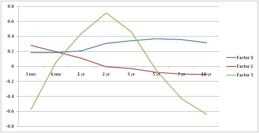
Components usually have particular shapes. In many studies the first component has been found to be fairly flat and therefore is representative of a parallel shift in the term structure. The second component is found to be downward sloping which causes the term structure to tilt or slope. The third component usually has a hump which accounts for the curvature in the term structure. There are other higher order components, but these first three components usually account for around 90%-95% of the variability in the term structure, so the other components are usually considered as noise and eliminated from further analysis of the components.
The relative importance of each component is assessed by the magnitude of the corresponding eigenvalue or rather the proportion of the eigenvalue relative to the sum of the eigenvalues of all the components.
Here is the output from our model after completing the PCA analysis of the US treasury curve data. The output will now be used as an input to the HJM interest rate forecasting model. Factor 1 refers to the level (or the parallel shift), Factor 2 refers to the slope and Factor 3 refers to the curvature (or the relative shift between intermediate rates and longer rates) across the term structure.