
The correlation coefficient is a measure of the strength and direction of a linear relationship between two variables. It may be calculated using the following formula:
Where
- n is the sample size
- xi is the measurement for the ith observation of variable x
- x_bar is the mean of all the observations of variable x
- σx is the standard deviation of the observations of variable x
- yi is the measurement for the ith observation of variable y
- y_bar is the mean of all the observations of variable y
- σy is the standard deviation of the observations of variable y
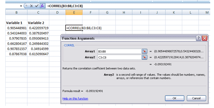
Alternately, it may be calculated in EXCEL using the function CORREL():
If you have more than two sets of data time series, i.e. variables, you may also generate a correlation matrix for the entire set of variables using the Data Analysis functionality of EXCEL:
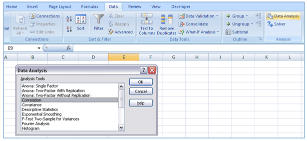
Step 1: Data Tab> Data Analysis>Correlation – Click OK
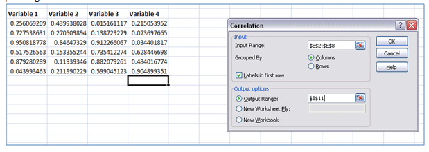

Step 2: Enter input range, check labels in the first row (if heading selected in input range) and specify output range – Click OK
The resulting correlation matrix is as follows:
The correlation coefficient, r, can range from -1 to +1 inclusive. The strength is gauged from the absolute magnitude of r, the greater the absolute value of r the stronger will be the relationship between the two variables. The direction is represented by the sign of the correlation coefficient- a negative sign representing negative correlation; a positive sign indicating a positive correlation. A value of r of -1 or +1 signifies perfectly negative or positive linear correlation respectively. A correlation coefficient of zero indicates that the two variables are not related.
Correlation coefficient assumes that the underlying variables have a linear relationship with each other. When the underlying relationship is non-linear then the correlation coefficient could lead to false and misleading results. Correlation could also lead to misleading results when there are outliers in the dataset, when data groups are combined inappropriately or when the data is too homogeneous.
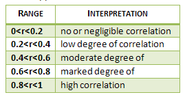
One way of interpreting the strength of the correlation coefficient is by using the following “Rules of Thumb” applied to the absolute value of the calculated measure:
In order to test whether the correlation is in fact significant rather than a chance occurrence we have used hypothesis testing. Specifically, we are testing the mutually exclusive hypotheses:

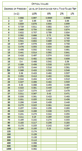
Using a significance level of 5%, a two tailed test and n-2 degrees of freedom (df) (n is the number of observations), a critical value is determined from the table below. If the exact degrees of freedom is not available in the table then the critical value at the next lower degrees of freedom will be used. For example, if there are 328 observations, degrees of freedom work out to 326. This value is not present in the table and so we will use the critical value at the next lower degrees of freedom, i.e. the critical value at degrees of freedom of 300.
If the calculated correlation is greater than the critical value or less than -1×critical value, it can be concluded that the calculated correlation is not a chance finding but is statistically significant. As a result, we reject the null hypothesis and accept the alternative. On the other hand, if the calculated correlation is less than the critical value or greater than -1×critical value, then we will conclude that there is no proof of correlation given the dataset and parameters used.
It is important to note that the size of the sample used affects whether a specific observed result attains statistical significance. With very large sample sizes, low correlation values which are demonstrative of a weak relationship between the variables can turn out to be statistically significant. This doesn’t mean that there is a significant relationship between the variables but simply illustrates that the correlation is not zero. Practical significance of the result should be gauged by the observed strength of the relationship, i.e. by its magnitude.
Correlations may change over time. Therefore it is important to calculate the correlation coefficient measure for different analysis periods as well as for different window lengths. This is done to assess the stability of the numerical measure as well as to identify periods when the correlations broke down or changed. For example, an increased value of the correlation coefficient measure relative to what usually is expected to result may be an indication of increased systemic risk in the market.
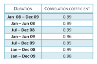
The following table shows the correlation coefficients for WTI and Brent spot prices calculated for various periods. We can see that the measure is relatively stable over time.
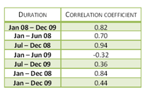
On the other hand, the table below shows the correlation coefficients for WTI and Steel spot prices calculated for periods similar to those used above. In this instance, we see that the measure varies considerably depending on the time frame over which correlations are evaluated.
