Pricing a financial instrument is not an exact science. There it is out there now; you can go ahead and lynch me for blasphemy.
While the formulae, the mathematics, the derivation, the proofs and the exact models would like us to believe otherwise, in essence pricing financial securities in these markets is more along the lines of a science of approximation. It’s a guessing game.
How do we approximate something for which we do not have a clearly defined underlying model? Sometimes we focus on behavior and build a symptomatic model – a model that under most conditions will approximate behavior and (we hope) pricing. In other instances we build model with their foundation in Economic theory – a game of supply and demand that theoretically indicates where a security would trade, if real world took its inspiration from a classical economic text book.
Both approaches demand an understanding of core price driving processes. The best approaches are a hybrid and then some. All approaches after a certain point in time need to dry run the model to see how it would behave under sets of assumptions, input factors and historical data sets.
Enter the simulation!
A simulation is an experiment. How will people react when you ring their door bell and run? Short of actually ringing the door bell and running do you have any other options? But sometimes ringing door bells and running is not possible in an academic or professional setting.
An easy compromise is a coin toss. In case of heads they will open the door, in case of tails they won’t. In case of heads they will scream and shout and curse, in case of tails they will quietly shake their heads and close the door. In case of heads the wrath of God will strike you down, in case of tails clouds will part, angels will sing and you will receive manna from heaven.
Over the last two centuries the science around coin tossing has been refined to mathematical poetry. All coin tosses are not created equal. Some lead to symmetry and are treated as fair. Other are clearly biased and are treated as skewed. Some come with memory (your result is dependent on the history of coin tosses), while others start afresh with each toss (as pure as driven snow).
So toss a coin a hundred times and if it is fair, you will travel the distance from the Binomial distribution all the way up to Normal. Toss it without memory and you can throw in the waiting game along with the Poisson analysis. Want a bit of a skew introduce the Lognormal, the Gamma and the Beta. The choice is yours but the results are very different.
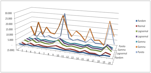
The graph that follows shows the result from a short simulation using some of the above mentioned distributions. While are distributions are equal, you can clearly see that some are more equal than others.
The art of using a coin toss to simulate the results of an experiment is one form of a simulation. Inspired by the ancient tradition of counting tosses and the close relationship between coin toss, cards and gambling the science is called Monte Carlo simulation.
What is a Monte Carlo Simulator
A Monte Carlo simulation at its heart is a simple coin tossing machine. Depending on the tool used to build the machine (the choice of distribution) the simulator will behave in a certain fashion (symmetric, asymmetric, normal and skewed, with thin tails or long fat tails).
MS Excel comes with its own built in Monte Carlo simulator. The simplest and easiest is the function called Rand(). The graph above was generated using the Rand() function embedded within MS Excel function calls to the Normal, Lognormal, Beta and Gamma distributions in MS Excel.
The choice of the underlying distribution is one of the primary factors in the model. The other drive is the model itself.
The process or generator function for the MC simulator – a first pass
Each MC simulation model comes with certain behavioral assumptions. These assumptions are based on process or what Nicholas Nassim Taleb (NNT) calls the generator function.
For instance let’s look at a simple function that calculates the rate of change in the price of a zero coupon bond on a continuously compounded basis. The generator function for bond prices will simply give you the change in bond prices every time you call it. You pick up the phone and dial the generator function, the generator function give you the change in bond price in return. The bond price you get would be based on three key factors.
- The principle invested in the bond
- The interest rate at which interest is being accrued
- The unit of time over which interest is being calculated.
How would you write this in the world of Monte Carlo Simulators? Don’t go into shock as yet, there is a simple key for this equation:
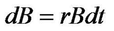
In the equation above:
dB = the rate of change in bond price
r = the rate of interest at which interest is being accrued
B = the principal invested in the bond at inception or time zero
dt= is the unit change in time
If you solve this equation for the rate of change in bond price, you can actually calculate the bond price at any given point in time.
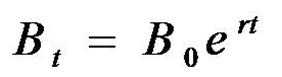
How do you read this? The value of a Bond B at time t (Bt)
is equal to the initial principal invested at time zero (B0)
continuously compounded at the interest rate r for time t. ert represents the continuous compounding at interest rate r for time period t function. If you were to plot this it would look something like the graph that follows:
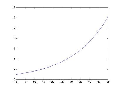
Congratulations you have just deciphered your first generator function. If you were to go back you would see that the function had three primary components. An equation that described the change in bond prices from one node in time to the next (the dB equation), an equation that described the full price at any given point in time (the Bt equation) and a graphical simulation of the model that showed how bond prices would change over a period of time across different yields.
Building your first Monte Carlo (MC) Simulator model
The first MC simulation model that we have built above has one basic flaw. There is no uncertainty. Prices will change when you change rates or maturity but other than that there is really nothing to simulate. It is a great model for introducing us to the terminology of Monte Carlo simulators, but it is not really a simulator. It’s simply a static pricing function.
So how do we build on what we have to create a Monte Carlo simulator?
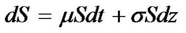
Here is a slightly revised model for calculating the change in price of an equity security.
Comments are closed.