Computational Finance: Building your first Monte Carlo (MC) simulator model for simulated equity prices in Excel

4 mins read

Building your first Monte Carlo (MC) Simulator model

The first MC simulation model that we have built above has one basic flaw. There is no uncertainty. Prices will change when you change rates or maturity but other than that there is really nothing to simulate. It is a great model for introducing  the terminology of Monte Carlo simulators, but it is not really a simulator for financial securities. It is a static pricing function that allows us to take the first step in defining what Nassim Taleb calls a generator function and helps us better understand the elements of uncertainly that we have to model by cleanly separating it from the static, known piece of price variation dependent on interest rates (or the risk free rate or the expected return depending on the model of your world) and time.

How do we build on what we have done so far to create a Monte Carlo simulator for financial securities?

Let us start with the financial security we are all comfortable with. A listed equity instrument that trades on an exchange. Here is a slightly revised model for calculating the change in price of an equity security. We now add one more component to our generator function. While the first term works off expected return the second term will help us model uncertainty.  Since in our world we drive and link uncertainly with volatility, our model also uses a factor proportional to volatility. Proportional in the sense that a stock priced at 10 with 20% volatility will see 3 sigma price variations of +6 and -6, while a stock priced at 100  will see +60, -60 movements for the same parameters.

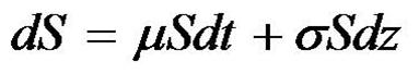
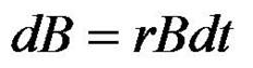
While the equation looks a little bit more complex than the rate of change in bond price equation above (and below) the form of the factors is similar. Rather than the risk free rate r we have u, rather than B we have S.

But in addition to the single static factor that this model has in common with bond pricing, there is one more change. There is a new factor which at first glance looks similar but required a slightly more detailed review.

Let’s take another look

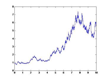
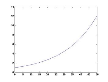
Rather than r or u we have sigma and rather than dt we have dz. Before we try and understand what these changes represent let’s take a look at the graphical model output above, side by side with the bond pricing model. As you can see below, that the clean, smooth bond pricing curve has been replaced by a jagged, volatile (some would say violent) trend. And since the shape and form of the first factor is similar to the bond pricing equation, this must be the work of the second factor.

The dz term that we have added above represents uncertainty. It’s random sample from a normally distributed simulator that is then scaled by the size of volatility or sigma. So what that basically means for the equation above is this:

The change in price of the stock price is comprised of two factors. A static return in proportion to the price of the equity security as well as the expected return (also known as drift) and the scaled volatility into a normally distributed uncertainty element. When we solve this we get the following equation

Similar to the bond pricing solution, this solution comes with a similar interpretation. The change in price from one period to the next is proportional to the original price times a factor. The factor is based on the expected return (adjusted for the volatility drag – the half sigma square) and the scaled volatility times an uncertain component.

This simple two factor base line model is the heart of Monte Carlo simulators and rate generators for equities, currencies, commodities and other non-interest bearing securities. Drift and Diffusion; expected return and volatility, mu and sigma. The first term (factor) is certain and will not change from one iteration to the next, the second one is not.

Here is a simple excel worksheet that implements this MC simulation model. The first table shares the numerical result from the MC simulation. The second exposes the underlying formula behind the calculations required for the MC simulation. For these results we have assumed that:

Spot price at time zero = S₀ = 30

Constant Volatility = sigma = 50%

Time to Maturity = T = 1

Risk free discount rate = r = 1%

The process used to create the Monte Carlo simulation worksheet in Excel using the projected price Monte Carlo simulation equation

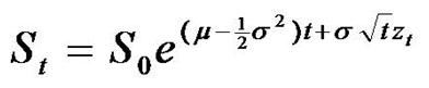
is as under:

The Monte Carlo Simulation Numerical Example in Excel Walk through

1. Monte Carlo Simulation – Column one – Generate a series of random numbers by using the Excel RAND() function. This series is a uniformly distributed series with random values fluctuating between 0 and 1.
2. Monte Carlo Simulation – Column two – Convert the uniform distribution series in column one to a normally distributed series by using the Excel function NORMSINV(). The NORMSINV function takes in a probability estimate (a number distributed between 0 and 1) and transforms that into a normally distributed series between +X and –X.
3. Monte Carlo Simulation – Column three – Calculate the first part of the equation (mu – .5 sigma squared) by replacing mu by r, the risk free rate. Remember that we are assuming a risk neutral world as far as this simulator is concerned under the Black Scholes assumptions which implies at all assets grow at the risk free rate.
4. Monte Carlo Simulation – Column four – Calculate the second part (the uncertain part) of the equation.
5. Monte Carlo Simulation – Column five – Calculate the change in previous price by combining the certain part with the uncertain part.
6. Monte Carlo Simulation – Column six – Calculate the new stock price.

The associated formula for the Monte Carlo Simulation are given in the next figure.

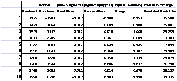
Figure 1 MC Simulation – Numerical results

The Monte Carlo Simulation Numerical Example in Excel Walk through – Spreadsheet formula

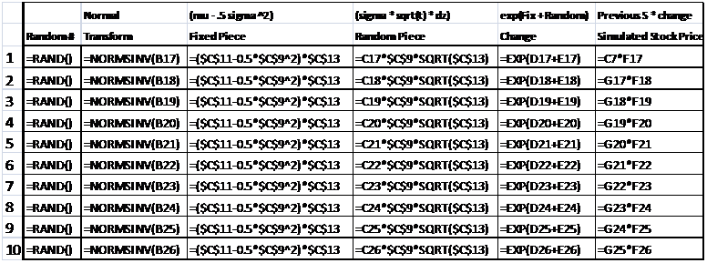
Figure 2 MC Simulation – Excel Formula