Here is the cosmic code joke again. If you can read this, you will understand perfectly what the following section on calibrating the CIR (Cox, Ingersoll and Ross) model means. If you can’t you still have to take that course on computational finance. Now without further ado, here goes:
1. The interest rate series (rt*) is obtained for the given benchmark yield curve.
2. A centered CIR model is obtained. This is done by subtracting the rates at each data point with their long run average (γ) across the entire series to obtain a transformed series (rt).
rt= rt*- γ
where the Centered CIR model used is
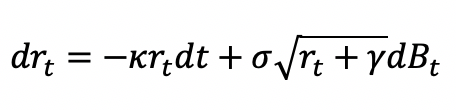
and κ is the continuous drift term & σ is the continuous volatility term.
3. The least squares method is used to estimate the parameters for the discrete representation for the CIR model using the Simple Discretization process. This is done as follows:
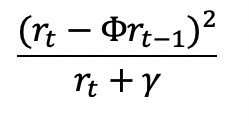
a. At each data point the following residual term is calculated:
i. For Simple Discretisation
ii. For Covariance Equivalent Discretisation
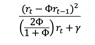
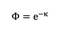
Where φ is the discrete drift term.
b. Calculate the residual sum of these terms across all data points (RSS)
c. Using the solver function minimizing this RSS term by changing the value of the discrete drift term, i.e. φ
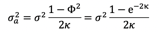
The least squares estimate of the discrete volatility parameter σa is given by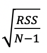
where N is the number of residual terms.
4. These parameters are then transformed to the continuous form as follows:
- Continuous drift, κ
- Continuous volatility, σ
Based on the CKLS Paper on calibration of Interest Rate Models aka
The K.C. Chan, G. Andrew Karyoli, Francis A. Longstaff and Anthony B. Sanders (1992)
The Volatility of Short-Term Interest Rates: An Empirical Comparison of Alternative Models of the Term Structure of Interest rates