The option adjusted spread (OAS) is a constant spread that when added to the interest rates used to discount the cash flows produces a theoretical value of the bond that is equal to the market price of the bond. It is an alternative way of expressing the difference that lies between the theoretical value and the observed market price, i.e. in the form of a yield spread rather than a difference in prices.
1. OAS model process for mortgage pass through security
In order to demonstrate how the OAS is determined for the Mortgage Pass Through Security in our model we have followed the steps given below:
- For illustration purposes, the observed market price is assumed to be the value of the MBS calculated using a constant discount rate equal to the 30-year fixed mortgage rate observed in the market assuming prepayments occur at 100% of PSA.
- We use an OAS Monte Carlo simulation approach to generate 100 interest rate paths. These interest rates are assumed to be short term rates to which the OAS is added to determine the rates at which MBS cash flows will be discounted. The simulated interest rates are also used to determine the prepayment rates for the MBS.
- In order to determine the relationship between the prepayment rates and the interest rates, we have developed a prepayment rate function which is a function of interest rates using linear regression and based on the historical relationship between these two rates.
- Based on the simulated rates the future Mortgage Pass Through cash flows for each interest rate path are calculated. The cash flows are discounted by interest rates plus a “guess” OAS to determine 100 theoretical prices for one unit of Mortgage Pass Through Security.
- A simple average of the theoretical price over all paths is calculated and the model solves for an OAS that equates this average simulated price to the observed market price.
2. A Simplified Numerical Finance Calculation Example for Option Adjusted Spread
It is assumed that the observed market price of a mortgage pass through security is 2,488.93. The mortgage pool underlying this security comprises one 1-year mortgage of 100,000 with a contract rate of 4.56% and a service fee of 0.5%. The cash flows of the underlying pool are distributed among the units of the MBS on a pro rata basis. There were 40 units of the MBS issued.
a. Project spot rates
In order to determine the Option Adjusted Spread (OAS) for the security we first project spot interest rates which together with the OAS will be used to discount the cash flows of the underlying security.
Let us assume that our model consists of two simulated interest rate paths as follows (the rates are spot rates quoted on an annual effective basis):
| Month | Projected Interest Rates Path 1 | Projected Interest Rates Path 2 |
| 1 | 4.20% | 4.26% |
| 2 | 4.17% | 3.87% |
| 3 | 4.08% | 3.93% |
| 4 | 4.06% | 4.05% |
| 5 | 4.06% | 4.08% |
| 6 | 4.17% | 4.13% |
| 7 | 4.03% | 4.13% |
| 8 | 4.04% | 4.15% |
| 9 | 4.10% | 4.17% |
| 10 | 4.04% | 4.17% |
| 11 | 4.04% | 4.15% |
| 12 | 4.07% | 4.16% |
b. Projecting prepayment patterns
The interest rates will not only be used in the determination of the discounted values of the cash flows, but they will also be used in determining the future pattern of prepayments which are assumed to be a function of these interest rates. These prepayment rate projections are expressed as a percentage of the PSA model. The derived PSA and prepayment rates under path 1 are given below:
| Month | x% of PSA | Prepayment Rates* |
| 1 | 215% | 0.43% |
| 2 | 218% | 0.87% |
| 3 | 227% | 1.36% |
| 4 | 230% | 1.84% |
| 5 | 230% | 2.30% |
| 6 | 219% | 2.62% |
| 7 | 233% | 3.26% |
| 8 | 232% | 3.71% |
| 9 | 225% | 4.06% |
| 10 | 231% | 4.62% |
| 11 | 231% | 5.09% |
| 12 | 228% | 5.48% |
*For simplicity, in this example, we assume that defaults are negligible.
c. Calculating the cash flows
We now determine the cash flows of the underlying mortgage pool. These detailed scheduled and unscheduled payments under the loan for interest rate path 1 are given in the table below:
| Month | No. of Loans |
Beginning Mortgage Balance |
Monthly Mortgage Payment |
Net Interest Payment For the Month |
Servicing Fee | Principal Repayment |
Prepayments | Ending Mortgage Balance |
| 1 | 1.00 | 100,000.00 | 8,540.60 | 338.33 | 41.67 | 8,160.60 | 32.97 | 91,806.43 |
| 2 | 1.00 | 91,806.43 | 8,537.53 | 310.61 | 38.25 | 8,188.67 | 61.06 | 83,556.70 |
| 3 | 1.00 | 83,556.70 | 8,531.30 | 282.70 | 34.82 | 8,213.78 | 86.23 | 75,256.69 |
| 4 | 1.00 | 75,256.69 | 8,521.53 | 254.62 | 31.36 | 8,235.56 | 103.59 | 66,917.54 |
| 5 | 1.00 | 66,917.54 | 8,508.36 | 226.40 | 27.88 | 8,254.07 | 113.60 | 58,549.86 |
| 6 | 0.99 | 58,549.86 | 8,491.89 | 198.09 | 24.40 | 8,269.40 | 111.21 | 50,169.25 |
| 7 | 0.99 | 50,169.25 | 8,473.10 | 169.74 | 20.90 | 8,282.46 | 115.54 | 41,771.25 |
| 8 | 0.99 | 41,771.25 | 8,449.73 | 141.33 | 17.40 | 8,291.00 | 105.26 | 33,374.99 |
| 9 | 0.99 | 33,374.99 | 8,423.16 | 112.92 | 13.91 | 8,296.34 | 86.37 | 24,992.28 |
| 10 | 0.98 | 24,992.28 | 8,394.15 | 84.56 | 10.41 | 8,299.18 | 65.73 | 16,627.37 |
| 11 | 0.98 | 16,627.37 | 8,361.10 | 56.26 | 6.93 | 8,297.92 | 36.17 | 8,293.28 |
| 12 | 0.97 | 8,293.28 | 8,324.79 | 28.06 | 3.46 | 8,293.28 | 0.00 | 0.00 |
The project cash flows for 1 unit of MBS for the two interest rate paths are given below:
| Month | Mortgage Pass-through Cash Flow for Path 1 | Mortgage Pass-through Cash Flow for Path 2 |
| 1 | 213.30 | 213.27 |
| 2 | 214.01 | 214.22 |
| 3 | 214.57 | 214.70 |
| 4 | 214.84 | 214.82 |
| 5 | 214.85 | 214.79 |
| 6 | 214.47 | 214.48 |
| 7 | 214.19 | 214.02 |
| 8 | 213.44 | 213.29 |
| 9 | 212.39 | 212.34 |
| 10 | 211.24 | 211.18 |
| 11 | 209.76 | 209.80 |
| 12 | 208.03 | 208.16 |
d. Discounting the cash flows & solving for OAS
The projected interest rates plus a “guess” OAS are used to discount the cash flows to determine the theoretical price. Once the price is determined under the various interest paths, the model solves for the OAS that makes the average of the theoretical prices equal to the observed market price. In our example, this works out to an OAS of 0.9035% p.a.
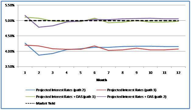
e. Comparison – Spot Rates vs Interest Rates plus OAS vs Market Yield
The comparative view of the projected spot interest rates, interest rates plus OAS and market yield is depicted below:
3. Implied Option Cost
The implied option cost is the difference between the OAS and a static spread. The static spread is the spread that an investor would earn if there were no changes in the current interest rate environment. The OAS, on the other hand, reflects the uncertainty present in future interest rates and hence the uncertainty in future cash flows due to the homeowner’s option to prepay. It is, therefore, less than the static spread as it adjusts for this option.
a. Methodology for calculating static spread
One way of calculating the static spread is to
- discount the future cash flows using the current zero curve plus a spread applicable to the entire theoretical spot rate curve (i.e. a “guess” static spread), and
- keep the future mortgage rates fixed at the current mortgage rate, in other words assuming that prepayments remain at levels seen at current mortgage rate. We have assumed that based on the current mortgage rate the prepayments will remain at 178% of PSA for the tenor of the loan.
Based on the prepayment assumption we calculate the future cash flows and discount them using the current zero rate curve plus the spread as given below:
| Month | Current zero rate curve | Mortgage Pass- through CF |
| 1 | 3.91% | 213.16 |
| 2 | 3.91% | 213.74 |
| 3 | 3.90% | 214.14 |
| 4 | 3.92% | 214.35 |
| 5 | 3.94% | 214.38 |
| 6 | 3.96% | 214.21 |
| 7 | 3.98% | 213.86 |
| 8 | 3.99% | 213.31 |
| 9 | 4.01% | 212.58 |
| 10 | 4.02% | 211.65 |
| 11 | 4.04% | 210.53 |
| 12 | 4.05% | 209.22 |
The static spread is solved for the spread that equates the discounted cash flows to the market price. In our case, this works out to a static spread of 1.0083%.
The implied option cost, therefore, works out to 0.1049% (=1.0083%-0.9035%).
Comments are closed.