Of all the intimidating equations and formulas (PDE’s and otherwise) out there, the derivation of the Black Scholes Model formula for a European option easily takes first prize for the most un-approachable of topics for new arrivals in this field. For many of us, it is literally a one way conversation with Greco Roman symbols. If the terminology doesn’t kill you, Itto’s Lemma will.
I have now been teaching executive MBA students for a while and have searched in vain for a treatment that is less shocking to the system at 9 pm in the evening. This year I finally decided to write one.
I couldn’t escape the equations or the mathematics involved completely but I have tried to keep it basic and concise. The objective is not to drive the equation but simply get more comfortable with the intuition behind it. From a presentation point of view, I have taken a lot of liberties to simplify the content. While I will certainly fail my Ph.D. review, the dumbed down end result is possibly a little easier to digest for a typical business school and computational finance student.
The inspiration for the treatment goes back to Maria Vassalou and Mark Broadie who first introduced me to it at Columbia. Maria did the theoretical introduction to Lars Tyge Nielsen’s framework while Broadie blew away any inhibitions we may have had in converting that into a workable EXCEL spreadsheet. The remaining bridges were built by my students in Dubai and Singapore where we walked through the finer points of the framework as part of the coursework for the Financial Derivatives and Risk Management courses.
a. Objectives
The objective of this note is to answer some very basic questions:
- What is the setting and context for the Black Scholes Model formula?
- What is the easiest and simplest way for deriving N(d2) that does not require half a text book on the mathematics of computational finance?
- If you are appearing for a Quant interview tomorrow morning and worry about your relationship with the Black Scholes Model, what can you do in 66 minutes to improve your probability of survival?
The treatment is based on material presented in Lars Nielson’s excellent and highly recommended text book on the subject and Maria Vassalou’s teaching notes (Continuous Time Finance seminar) from her days at Columbia Business School.
b. Underlying Assumptions
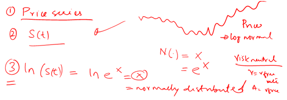
Within the Black Scholes Model world, we assume the following for the underlying distribution for S(t) and ln (S(t))
There is an available price series of non dividend paying financial security given by S(t). We assume that S(t) is distributed log normally which simply means that if Y represents the price series and X represents a normally distributed random variable then:
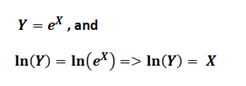
The take away from the above equations is that while S(t) is log normally distributed, ln(S(t)) is normally distributed.
We also assume that the standard deviation and expected return for ln(S(t)) is given by:

Why the risk free rate? Because in the risk neutral world, investors are content with earning the risk free rate and all assets earn the risk free rate. (T-t) will get simplified to just t in our illustrations that follow.
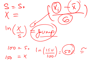
c. Estimating the jump
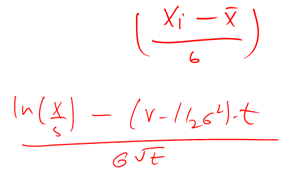
For a European call option, we know that the option will only be exercised if the terminal price S(t) is greater than the strike price X. Therefore, the first probability of interest is the probability that S(t) >= X or N(d2). But to calculate the probability for our series, (remember we are dealing with ln(S(t)) and not S(t)), we first need to convert our series to a standard normal distribution and estimate a Z score.
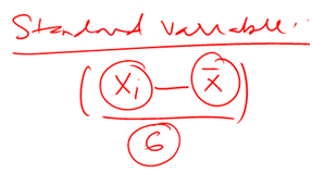
The Z score is basic statistics. As long as we have the value that needs to be compared, the mean and the standard deviation of the distribution we can simply plug them in the equation above. Mean and standard deviation we already have (see above discussion), the value that needs to be compared is the jump. How high does S need to jump for the option to be in the money? We need to, therefore, compare the original spot price (S nought) with the Strike (X) to calculate the size of the jump. We use the natural log approximation to estimate the magnitude of the jump.
Once we have the Z score, calculating the probability is a simple call to the Normal distribution function in EXCEL.
d. Plugging in the values in the Black Scholes d2 formula
We now take our estimate of expected return and standard deviation and plug it in the standard normal conversion equation and get the following results
But before our work is complete we need to make a tweak.
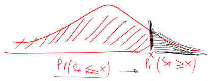
The standard normal distribution we have used above calculates the probability of S(t) < X, while we need S(t) >= X. It’s not a big hurdle. All we need to do is rather than use the Z score, d, use (-d) and our job is done.
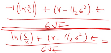
We multiply our result above with (-1) across and simplify to our now very familiar value of d2.
e. Black Scholes Model – Video Series
If you would prefer to follow the above discussion using a video format for better understanding, here is the series:
There are four videos in the series. The first two present a theoretical review (read: boring and sleepy). The next two review a simple Excel model we put together to make it easy to visualize Lars’ framework.
Video 1
The first video in the understanding Black Scholes Model series reviews the intuition behind N(d2). Essentially the same material you read above delivered in my soothing, sing song voice. (Time – 20 minutes).
Video 2
The second video in the series looks at extending that intuition to building EXCEL based simulators for simulating financial securities. Once you have reviewed the videos you are now ready to understand the difference between N(d1) and N(d2). (Time – 19 minutes)
Video 3
You are now armed with sufficient knowledge to be dangerous with an EXCEL spreadsheet. The third video walks you through the structure of a simple Monte Carlo simulator model to simulate a financial security. Please note that we don’t walk through the actual model building process, just the model. If you have been diligently following us so far, the model building piece shouldn’t be that difficult. If you still need help, drop me a line and I can share a few more useful hints and tips. (Time – 10 minutes)
Video 4
The fourth and final video uses this simple model to reinforce the concepts we have just discussed. Specifically, the intuition behind the two probabilities – N(d1) and N(d2). And a special focus on the variations around S(t) > X – or the terminal S being greater than the strike price. (Time – 15 minutes)
Enjoy.

Comments are closed.