Monte Carlo Simulation Model – How To – Simulating Crude Oil Prices
To simulate crude oil prices we will follow a multi step process. We first present the input required and output produced from the simulation model and then follow with a step by step review of the model building process.
Please make sure that before you proceed, you have reviewed the relevant background material and theoretical review of Monte Carlo Simulation provided on the primary Monte Carlo Simulation Models page.
Monte Carlo Simulation Model – Specification
To begin we need values for the following parameters.
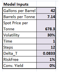
The target output is a monthly series of simulated crude oil prices per tonnes.
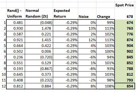
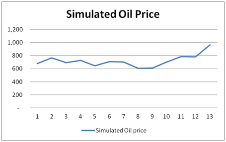
The rational, the model & the parameters are discussed separately on the Monte Carlo Simulation Resource page. But briefly we use expected return as a fundamental driver of value and add simulated noise to model random movements in prices. Return is constant as per the original model specification while noise is random and changes from one simulation to the next. The last shaded column provides the final model output which is also plotted using a line graph.
Monte Carlo Simulation – Simulating Normally distributed Random Numbers
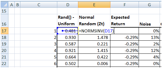
We can use Excel’s RAND() function to generate a uniformly distributed random number between 0 and 1. Column D (the first column) in our model below does just that. However for simulating a financial security, commodity, equity or currency we need a normally distributed random number. We can calculate that by calling the NORMSINV function. The input to the function is a number between 0 and 1, which is provided by our first call to the rand() function in cell D. The input signifies probability and the output is a normally distributed random number from a normal distribution with mean zero and standard deviation one.
The normally distributed random number will be used later in simulating noise/error/uncertainty in the model. A quick note, your numbers will not match these numbers since our laptops will use a different seed for the random number generator.
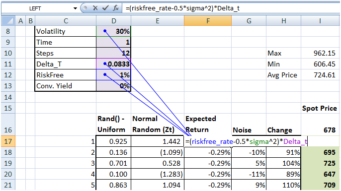
Monte Carlo Simulation Model – Calculating Expected Return
The next column (column F) calculates expected return by using the risk free rate, volatility and the first time step (small t or delta_t). Since all three parameters are constant, the value will remain the same across all iterations. We have used a step by step break down so that you can follow the process. However generally the five columns presented below can easily be compressed in one.
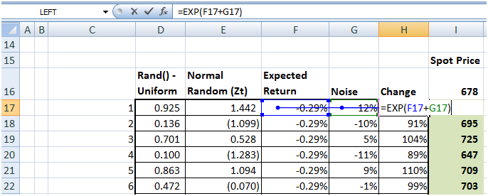
Monte Carlo Simulation Model – Calculating Random Noise
The original model specification uses a constant expected return (above) and a simulated error term (uncertainty below) to estimate the change in the value of the simulated security from one time step to the next. We multiply standard deviation for the period – sigma* sqrt (delta_t) – with the normally distributed random number to get the uncertain element in our equation.

Monte Carlo Simulation Model – Estimating simulated change in prices
Our last step is estimating the change and using that change to calculate the simulated price for the period. Once we have completed this exercise for the first row, all we have to do is copy and paste the relevant cells all the way to the 12th row and the first pass on the model is complete.
The last cell at Column I, Row 28 (962) has the number that we need, which is the simulated price of crude oil per tonne.
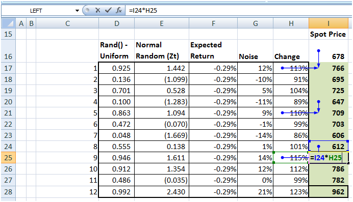
The challenge however is that this value by itself is of limited use because it changes from one iteration to the next. To complete our simulation exercise we must store this result in a data table and average it out over 500 to 5,000 simulations.
But rather than doing this here, we will build our data table and results warehouse, when we have a few more items to store in our next post.
Comments are closed.