Solver Functionality and Workaround
A key element in the construction of the Black Derman Toy interest rate model is the setting up and running of EXCEL’s Solver function. The Solver functionality links various parts of the model together, the inputs- initial zero curve rates and their volatilities, the calculation cells – price lattices and short rate tree, and the output cells – median rates and sigmas that are used to construct the short rate tree which is used in bond pricing. When the Solver function is run successfully the outputs produced by the model will be calibrated to the current term structure of the zero rate curve as of the valuation date thus ensuring that there are no arbitrage opportunities possible and also that the model is marked to market.
Issue #1: Excess of adjustable cells
However, EXCEL’s standard solver functionality is limited in that it can only work for a given number of adjustable cells. Solving for median rates and sigmas with constraints on prices and/ or volatilities over a long duration such as thirty years or a greater frequency such as quarterly or monthly time steps will often times be beyond EXCEL’s current capability resulting in the failure of the Solver function to run.
Issue #2: Cannot find feasible solution or repeatedly returns an error
Another instance where the work around comes in handy is when despite the fact that the number of adjustable cells are manageable by EXCEL’s standard functionality, the Solver function returns an error or cannot find feasible solutions. This mainly seems to be due to the inflections in the initial volatility term structure.
Work around methodology
There are stronger optimization programs available or one may be developed from scratch, however there is a way that the Solver function within EXCEL’s limited framework may be used to solve for the median rates and sigmas of the BDT model in such instances. The question to answer when using this work around is “What is the objective of the Solver functionality with regard to the BDT model?” The answers could be either:
a) Ensure that prices from the lattice equal to the initial prices determined using the initial zero curve rates as well as ensure that yield volatilities from the price lattice equal the initial zero curve volatilities, OR
b) Ensure that prices from the lattice equal to the initial prices determined using the initial zero curve rates and that the differences between actual observed prices and model prices are minimized.
In short the work around must ensure that the primary constraint cells are satisfied and that target cell values (if not arbitrarily set) are reached.
The work around methodology uses a piece meal process. Set up the solver function for smaller portions of the data. For example, for a 10 year model with quarterly payment we may break up the period as follows: 0.25-3, 3-5, 5-7, 7-10.25 years. Smaller ranges may be chosen depending on whether Solver returns a repeated error message or larger ranges may be used if permitted. The ranges may be chosen at random or a more effective method of doing this, in particular if the calibration is of type (a) mentioned above, is to look at the term structure of the volatilities.
For example consider the following input cells for the BDT model:

Consider the graphical representation of term structure of the volatilities:
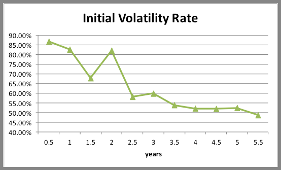
The volatilities fall between time steps 0.5-1.5, rise again at time step 2, fall again at 2.5, rise at 3 before exhibiting a downward trend for duration 3.5 to 4.5, rising once again at 5 and falling at 5.5.
In this instance we can use Solver in a piece meal fashion for the following ranges: 0.5-1.5, 1.5-2, 2-2.5, 2.5-3, 3-4.5, 4.5-5.5. Note that range boundaries are inclusive. This is important to ensure a smooth transition from one range to the next.
Concerns
It may be noted that such a methodology is time consuming, in particular if you are dealing with longer durations and smaller intervals. The process is one of trial and error with repeated manual resetting of the Solver function. Resetting in the first place because of the piece meal nature of the work around but also because there is a high probability that certain Solver runs may lead to errors in cells (#Num, #Div/0, negative values) leading to a failed attempt. In such instances you would, either have to choose smaller ranges or reset the cells and run the functionality again and continue doing so until Solver returns feasible results, or until the constraints seem to be adequately met.
Any change in the initial inputs or calculation cells (for change in frequency, tenor, etc) would mean that this lengthy process would need to be repeated.