The Black Derman Toy (BDT) model is a one-factor, no-arbitrage interest rate model. One-factor in that the entire term structure of interest rates can be inferred with reference to the process underlying the short rates derived. No-arbitrage in that the term structure derived is exactly consistent with the current term structure- the zero curve yield structure and their volatilities. The model’s output is calibrated to the current term structure to ensure that there are no possibilities for arbitrage and that there is a good fit.
To review the various types of interest rate models read the following course:
Interest Rate Simulation Crash Course
In general the inputs into a BDT model are the initial continuously compounded zero curve rates and their volatilities.
The zero curve rates may be derived from par yield rates. For our illustration we have obtained historical rates of US Daily Treasury Yield Curve Rates available on the US Treasury Departments website. We have assumed these rates are at par and we using the bootstrapping methodology to determine the zero curve rates. To review how to derive zero curve rates from the par term structure you may consider looking at the following posts:
Online Finance Course – Pricing Interest Rate Swaps – Fixing the term structure
Online Finance Course – Pricing Interest Rate Swaps – Calculating the zero curve
The zero rate derivation methodology above produces annual effective rates. To convert to continuously compounded rates we apply the transformation:
Continuously Compounded Zero Rate = LN (1+Annual Effective Zero Rate)
To calculate the spot rate volatilities we repeat the above process for a selected window of historical
YTM data. Once this has been done, for each tenor, we determine a returns series by taking the natural logarithm of the ratio of successive rates. We then calculate the standard deviation of this return series and scale it by number of (trading or calendar) days in a year to get annualized returns. Read more on how to calculate volatilities from historical time series data here.
Using a window length of 01-April-2013 to 29-April-2013:
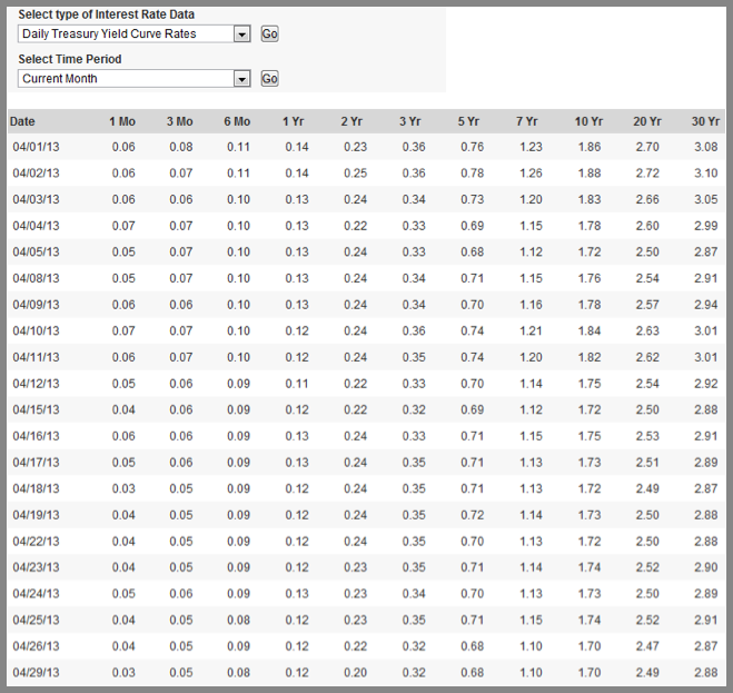
Source: US Department of Treasury (http://www.treasury.gov/resource-center/data-chart-center/interest-rates/Pages/TextView.aspx?data=yield)
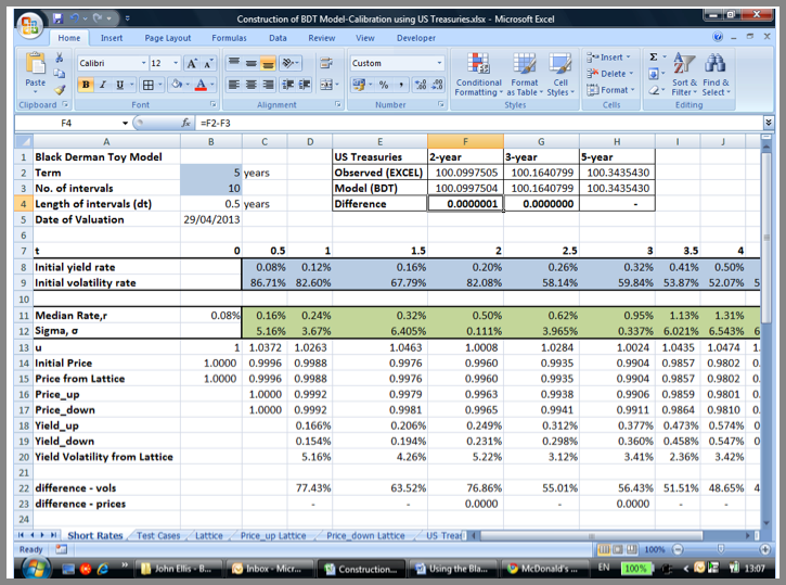
and the methodology mentioned above, we have derived the following input values for the BDT model:
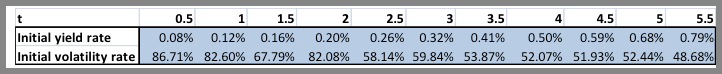
We have constructed the BDT model for semiannual frequency and for times 0.5 to 5.5 following the procedure outlined in the course:
How to build a Black Derman Toy (BDT) Model in EXCEL
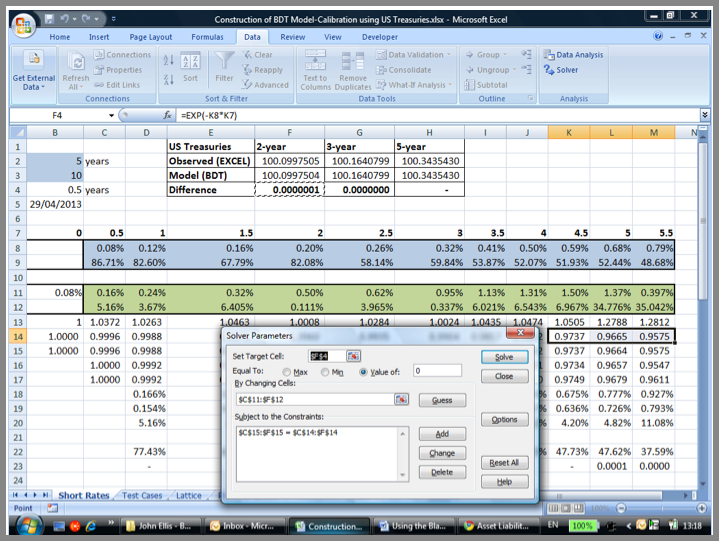
A vital element in the construction of the BDT model is the setting up and running of the Solver function in EXCEL. The result after the Solver functionality has been successfully run calibrates the model to the current/ initial term structure of zero coupon yield rates and their volatilities resulting in a no-arbitrage model. The original set up of the Solver function is:
- To maximize a target cell (an arbitrary cell that does not change in value as the solver runs through its various iterations), in our case the length of intervals cell, dt,
- By changing the output cells, the median rates and sigmas that are used in the calculation of BDT’s short rates tree
- And satisfying the following two sets of constraints:
- Prices determined from the BDT model’s price lattice = Initial prices determined using the initial zero curve yield rates
- Volatilities determined from the BDT model’s price lattices = Initial volatilities
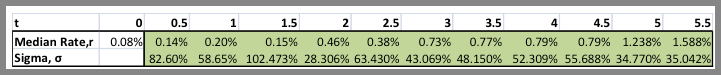
After running the solver function we arrive at the following output results for the median rates and sigmas that satisfy the defined constraints:
In order to test the calibration of the model, the output was then used to price 2-year, 3-year and 5-year US Treasury notes as of 29-April-2013. To review how the outputs of the BDT model may be used to price bonds refer to the following course:
How to utilize the results of a BDT interest rate model
The notes are assumed to have been issued on 29-April-2013 and have coupons rates of 0.25%, 0.375% and 0.75% respectively. Their observed prices are based on the YTMs for those tenors as at the valuation date (0.2%,0.32% and 0.68% respectively) and are calculated using EXCEL’s price function [i.e. PRICE(settlement date = 29-April-2013, maturity date = settlement date + tenor, rate = coupon rate, yield = YTM as at 29-April-2013, redemption =100, frequency =2 or semiannual and basis (day count convention) =1 or Actual/Actual)].
Observed and BDT model based prices are given below:
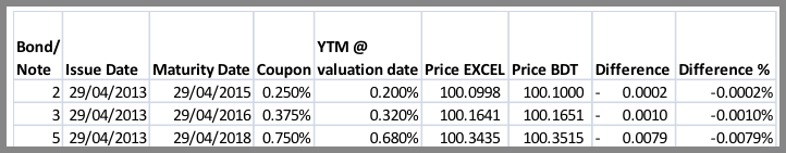
While the results produced by the model are relatively close to those observed, the BDT model is not exactly calibrated to US Treasuries as of the valuation date. If the model were used to price other fixed or floating rate instruments that are not as observable or liquid in the market as these Treasuries, it may lead to results that are not completely fair as the model has not been adequately marked to market in relation to observable and liquid market instruments.
One reason for the differences in prices could be that the initial volatilities used in the model are not consistent with the zero coupon rate volatilities implied in current bond prices. Remember that for the determination of the volatilities we have looked at a specific window of historical data. The volatilities are therefore a function of the data set used. If the window is changed the volatilities also will change accordingly. What then is the appropriate initial volatility term structure?
An alternate method of calibrating the BDT model to produce results that are consistent with current US treasury bond and note prices, is to calibrate the same to minimize the difference between the two sets of prices. The BDT model is constructed in the same manner as described above, but there are a couple of changes made to the way Solver is set up and run.
Prior to setting up Solver, it is important to call the results of the observed and BDT-model based prices to the same tab in EXCEL where the output results and constraint cells of the BDT model are present, otherwise Solver will not run. In our illustration we have two sets of prices for 2-year, 3-year and 5-year US Treasury notes:
Take the differences between these two sets of prices as shown is row 4, columns F, G and H above. We have used a 3 point calibration of prices but you may choose to use more or less accordingly.
The problem will now be set up in Solver for given ranges depending on the number of tenors (at which observed and model price differences are calculated) used for calibrating results. For each range the target cell for the Solver function will be different.
For the range 0.5-2 years the target cell will be the difference between the observed and model prices for the 2-year bond which will be set to a Value of Zero. This will be done by changing the median rates and sigmas for this tenor range while ensuring that the prices obtained from the price lattice equal the initial prices. Note that volatilities from the lattice are not constrained to the initial volatilities derived from historical time series data as before.
For the range 2-3 years we will set the target cell equal to the difference between the model and observed prices of the 3-year bond and for range 3-5.5 years we set the target cell equal to the difference between the model and observed prices of the 5-year bond. It is important to overlap the beginning and end duration selections from one range to the next to ensure a degree of smoothness in results. By its very nature the alternative calibration leads to model prices that match observed ones:
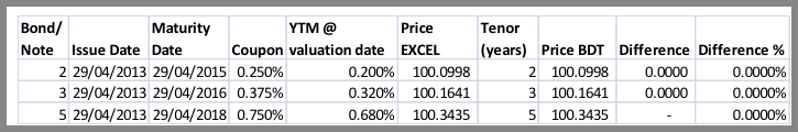
In this case we can truly say that the BDT interest rate model has been marked to market as of 29-April-2013, the valuation date.