We have introduced our friend mu (u) as drift and sigma as diffusion (or standard deviation or volatility or vol). In the previous session we have also gone out and built a simple excel based Monte Carlo simulation model for generating stock prices. While the process is focused right on equity securities, the same underlying structure, with some tweaks can be used to generate rates for currencies, commodities and interest bearing securities.
Let’s take another close look at our standard rate of change equation for a financial security
When we solve the equation above our solution looks something like this in a discrete form. In a risk neutral world, the risk free rate r takes over from mu (u).
Let’s do a simple experiment. We have two variables and four possible variations
| Mean (mu, drift, risk free rate r) | SD (Sigma, Diffusion, Vol) | |
| Zero drift, Zero vol |
0 |
0 |
| Unit drift, Zero vol |
1% |
0 |
| Zero drift, Unit vol |
0 |
1% |
| Unit drift, Unit vol |
1% |
1% |
Here are the graphical results from the same Monte Carlo Simulator we have built earlier. The simulated values have been plotted to give a more visual idea of the direction and trend of simulation results. The starting or initial spot price for the simulated security is 10.
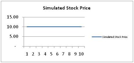
The Zero Drift, Zero Diffusion case
The first case is zero drift and zero volatility. The simulation plot is flat line going nowhere.
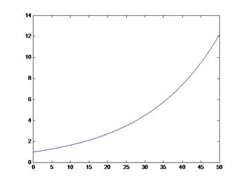
The Unit Drift, Zero Diffusion case
The second case is unit drift and zero volatility. The simulation plot is flat line going upwards. The unit drift grows the trend in a 45% angle line per unit of time and there is no uncertainty.
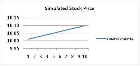
In some ways this is the same case as the exponential curve we saw earlier for bond pricing on a continuously compounded basis. There is a clear upward trend with no uncertainty or volatility.
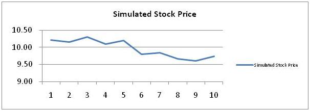
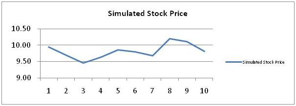
The Zero Drift, Unit Diffusion case
The third case is zero drift and unit volatility. And we can now see that while the overall trend is flat but there is now some uncertainty in results.
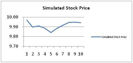
Within our Excel Monte Carlo simulator every time we press F9, the chart below will change and while there will be instances of directional trends (both upwards and downwards) a large majority of cases will have a flat trend with volatility.
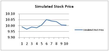
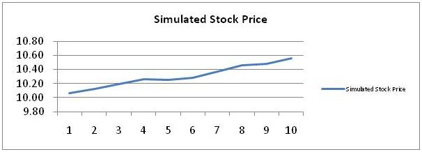
The Unit Drift, Unit Diffusion case
The final case is unit drift and unit volatility. A clear up trend is visible now. Once again while there may be some instances of downward and flat trends for these values, in a majority of cases the price trend will be upwards and positive.
Understanding Volatility drag or ½ sigma2
(squared)
Now what happens if we increase the drift to 5 units from the original one. You will see that the uptrend is now consistent across all iterations of your Monte Carlo simulation model. And the reason is that in our two factor model drift now dominates diffusion by the 5 times.
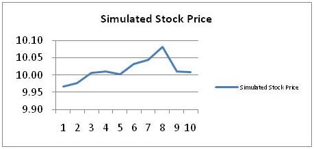
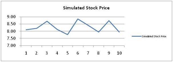
If you increase volatility in the same proportion to five units, we will still see a consistent up trend but every once in a while a high enough dz value will drag returns down as in the simulation results shows below.
As you carry on increasing volatility (to 10 units and then 25) in proportion to drift, the frequency of flatter and downward returns will increase.
This is the impact of the volatility drag or the subtraction of the
½ sigma2
(squared) term
in our Excel Monte Carlo simulation model.
fortunemaker:hey there, i’ve been looking fo a good price aoictn trading method for a while now and this seems like the real deal. i’ve seen day trade to win’s webinars about the ato trading es and atlas line but am considering the mentorship program. would love more info about that.thanks!