Greeks
Option Price Sensitivities (OPS) or Greeks measure how option prices change with respect to a specific pricing factor. The sensitivities are called Greeks because the five symbols used to represent the sensitivities are in Greek notation
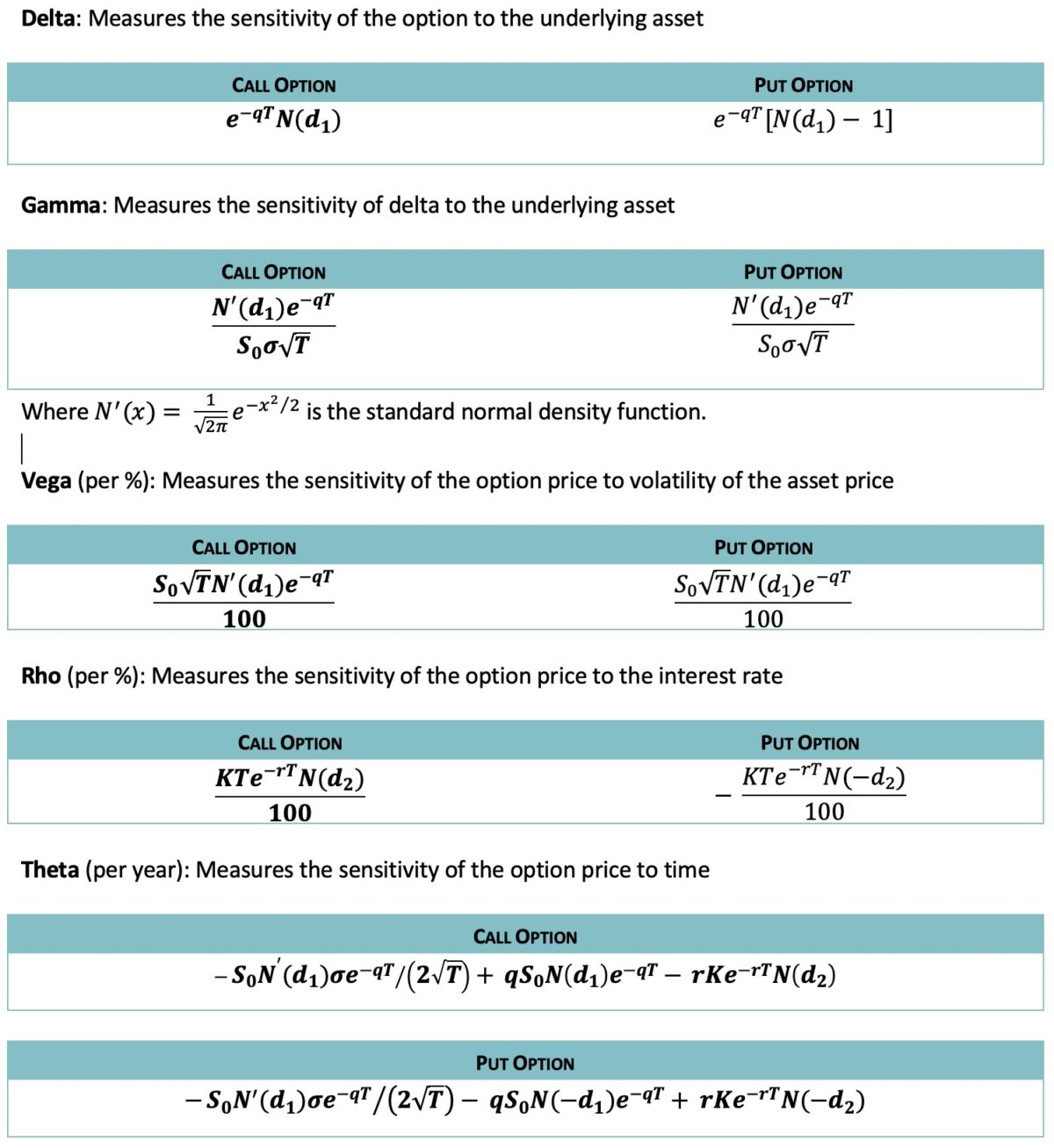
| Greeks | Factor | Comments |
| Delta | Change in option price due to change in the price of the underlying | First order change |
| Gamma | Change in option delta due to change in the price of the underlying | Second order change, think of it as a tool that measures convexity, the ability of an option to fall by less and rise by more. |
| Vega | Change in option price due to change in price volatility of the underlying | Volatility changes have a dramatic impact on price changes on deep out of money options |
| Rho | Change in option price due to change in the risk free rate | The relative impact of discounting and the tenor or maturity of option |
| Theta | Change in option price due to change in the risk free rate. | Think of this as the daily accrual that brings you closer to earning the premium every day. |
American option price
The American option price will be determined using a Binomial Tree. The steps in the calculation are as follows:
Step 1: Divide the specified time period of the option into n time steps with each step having length Δt. For example, if the life of the option is 30 days and the number of time steps is 5, Δt = (30÷5) ÷ 365 = 0.016438.
Step 2: Calculate the price at each node of the tree. At the node supposing the price is S. At the end of a time step the price will move up to Su with probability p and down to Sd with probability 1-p. Where,
In our example, we have considered a call option. The initial price is 100, the risk free rate is 10% and the dividend yield is 8%, the volatility is 20%, u = e0.20×?0.016438=1.0260,
Su = 100× 1.0260 = 102.60 and Sd=100/1.0260 = 97.47 and = 0.5
The prices at all the nodes will be as follows:
|
113.68 |
|||||
|
110.80 |
|||||
|
108.00 |
108.00 |
||||
|
105.26 |
105.26 |
||||
|
102.60 |
102.60 |
102.60 |
|||
100.00 |
100.00 |
100.00 |
|||
|
97.47 |
97.47 |
97.47 |
|||
|
95.00 |
95.00 |
||||
|
92.60 |
92.60 |
||||
|
90.25 |
|||||
|
87.97 |
|||||
Node Time: 0 |
0.01644 |
0.0329 |
0.0493 |
0.0658 |
0.0822 |
Step 3: Starting with the final node we work backwards to determine the option price or value at time 0. The option prices at the final nodes of the tree are the intrinsic values of the option.
At earlier nodes, we will first need to calculate a value assuming that the option is held for a further time step. We compare this value with the value if the option is exercised early. If the former value exceeds the latter the earlier exercise is not optimal. If the opposite is true the early exercise value will be selected for further stages in the calculation.
This is illustrated for our example below:
| B
13.68 | |||||
A | 113.68 | ||||
10.80 | |||||
D | 110.80 | C | |||
8.00 | 10.82 | 8.00 | |||
108.00 | 108.00 | ||||
5.26 | 8.04 | 5.26 | |||
105.26 | 105.26 | ||||
2.60 | 5.65 | 2.60 | 5.29 | 2.60 | |
102.60 | 102.60 | 102.60 | |||
0.00 | 3.80 | 0.00 | 3.29 | 0.00 | |
100.00 | 100.00 | 100.00 | |||
2.47 | 0.00 | 1.96 | 0.00 | 1.30 | 0.00 |
97.47 | 97.47 | 97.47 | |||
1.14 | 0.00 | 0.65 | 0.00 | ||
95.00 | 95.00 | ||||
0.32 | 0.00 | 0.00 | 0.00 | ||
92.60 | 92.60 | ||||
0.00 | 0.00 | ||||
90.25 | |||||
0.00 | 0.00 | ||||
87.97 | |||||
Node Time: 0 | 0.01644 | 0.0329 | 0.0493 | 0.0658 | 0.0822 |
The numbers above the prices (given in the boxes) are the value of the call option, i.e. max [Price –Exercise Price, 0] let’s call this O1.
For nodes 0 to 4 the values at the bottom represent the value of holding the option for a further time step, let’s call this O2.
O2 at A is (13.68*p +8*(1-p))/0.10 .The option value at the particular nodes will be the maximum of O1 and O2.
These are the values outside the boxes that are highlighted in the diagram above.
At A this is 10.82. O2 at D is (10.82*p +5.29*(1-p))/0.10 and so on. Following this process, the price of the call option is 2.47.
Comments are closed.