Here is a pricing and valuation equation glossary for the financial engineering field used as a reference for the courses posted on FinanceTrainingCourse.com. If you have come across a missing equation previously on a Learning Corporate Finance course, you will find it here.
For a complete reference to equations and calculator referred to in our course catalog, please see the Derivative Pricing and Financial Risk Equation Glossary.
For topic specific equations, please see the following links. For a list of topics covered under each of these links, please see the index below
- Calculating Value at Risk
- Duration, Convexity and Asset Liability Management
- Black Scholes, Derivative Pricing, Binomial Trees
- Calculating Forward Prices and Forward Rates
- Valuation of Interest Rate Swaps and Future Contracts
- Financial Risk, Reward metrics and measures
- Black Formula’s, Valuing Interest Rate Caps and Floors
Calculating Value at Risk
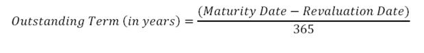
1. Outstanding term to maturity
(assumes Actual/ 365 day count convention)
2. Interpolation
(e.g. interpolation of rates between tenors t and t+1)
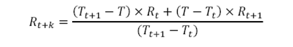
Where,
T= outstanding term = t+k years, where t≤t+k≤t+1 and 0≤k≤ 1
Tt=rounded down value of the outstanding term = t years
Tt+1= t+1 years
Rt=Rate observed at time t years
Rt+1=Rate observed at time t+1 years
Rt+k=Interpolated Rate for time t+k
3. EXCEL’s Price formula
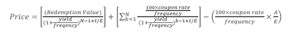
Where:
t = number of days from settlement to next coupon date.
E = number of days in coupon period in which the settlement date falls.
N = number of coupons payable between settlement date and redemption date.
A = number of days from beginning of coupon period to settlement date.
4. Continuous return of daily prices
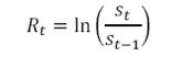
Where st is the price at time t and
Rt is the continuous rate of return of the daily prices and is calculated as the natural logarithm of successive prices.
5. SMA volatility (σ)
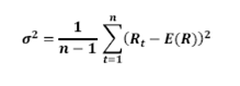
Where Rt is the rate of return at time t and E(R) is the mean of the return distribution, i.e.
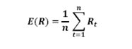
‘n’ represents the number of return observations used in the calculations.
6. EWMA volatility (σ)
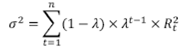
Where Rt is the rate of return at time t and
λ is the decay factor where(0< λ <1). The industry standard of λ is 0.94.
7. Weights and Scaling of weights under the EWMA approach
As per the EWMA VaR formula the weight for the data (return) point at time t is:
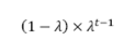
Where λ is the decay factor where(0< λ <1). The industry standard of λ is 0.94.
The sum to infinity of the all the weights is 1. However it is not possible to have infinite data so if the sum of weights is not close to one, certain adjustments are needed. One option is to increase the number of observations used in the data. The second option is to scale the weights by dividing each weight by the following factor:
![]()
Where n is the number of return observations.
8. Determining daily SMA and EWMA VaR
σ × z-value of standard normal cumulative distribution corresponding with a specified confidence level
9. Determining the index value for Historical VaR
Index Value = number of return observations × (1-confidence level%)
10. Scaling daily VaR
J-day VaR= √J × (daily VaR)
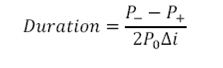
Duration, Convexity and Asset Liability Management
1. Duration
2. Convexity
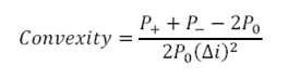
Where,
Δi= change in yield (in decimals)
P0= Initial Price
P+= Price if yields increase by Δi
P–= Price if yields decline by Δi
3. Approximate Price Change
Total estimated percentage price change= -Duration×Δi×100+Convexity×(Δi)2×100
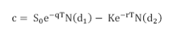
Black Scholes, Derivative Pricing, Binomial Trees
1. Black Scholes Formula
a. Call Option price (c)
b. Put Option price (p)
![]()
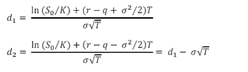
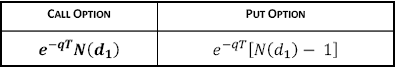
Where
N(x) is the cumulative probability distribution function (pdf) for a standardized normal distribution
S0 is the price of the underlying asset at time zero
K is the strike or exercise price
r is the continuously compounded risk free rate
σ is the volatility of the asset price
T is the time to maturity of the option
q is the yield rate on the underlying asset. Alternatively, if the asset provides cash income, instead of a yield, q will be set to zero in the formula and the present value of the cash income during the life of the option will be subtracted from S0.
2. Greeks
a. Delta
b. Gamma
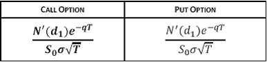
Where
![]() is the standard normal density function.
is the standard normal density function.
c. Theta (per year)
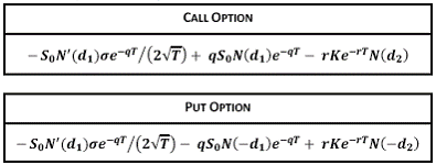
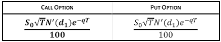
d. Vega (per %)
e. Rho (per %)
3. Binomial Tree
a. Probability
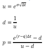
Where p is the probability that at the end of the time step, Δt, the price (S) will move up to Su. Alternatively 1-p is the probability that the price will move down to Sd.
r is the risk free rate
q is the dividend yield
σ is the volatility of the prices
b. Price at node
 c. Payoffs at nodes (1 step tree) – European Call Option
![]()
d. Price of a European Call option (1 step tree)
Price of the option (value at time 0) = Expected present value of payoffs = C=e-rΔt{pCu + (1-p)Cd}
Calculating Forward Prices and Forward Rates
1. Forward Price
a. Forward price of a security with no income
![]()
Where S0 is the spot price of the asset today
T is the time to maturity (in years)
r is the annual risk free rateof interest
b. Forward price of a security with known cash income
(Securities such as stocks paying known dividends or coupon bearing bonds)
Where I is the present value of the cash income during the tenor of the contract discounted at the risk free rate.
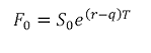
c. Forward price of a security with known dividend yield:
(Securities such as currencies and stock indices)
![]()
Where q is the dividend yield rate. For a foreign currency q will be the foreign risk free rate.
2. Spot Rates and Forward Rates
a. Relationship between spot rates and forward rates-1
![]()
b. Relationship between spot rates and forward rates-1
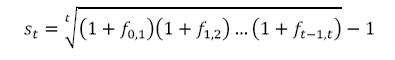
Where st is the t-period spot rate and
ft-1,t is the forward rate applicable for the period (t-1,t)
3. Yield to Maturity (YTM)
To solve for YTM we are solving for the interest rate (r) in the bond valuation formula:
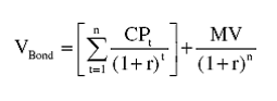
Where CPt is the coupon payment at time t and MV is the maturity value at time n (i.e. at maturity).
4. Forward Rate Agreement (FRA)
The value of the FRA at time 0, VFRA, for someone receiving fixed and paying floating will be
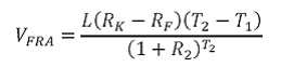
if R2 (the zero coupon rate for a maturity of T2) is calculated on a discrete basis or
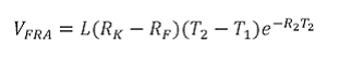
if R2 is calculated on a continuous basis.
Where, L is the principal amount
RK is the fixed interest rate
RF is the forward interest rate assuming that it will equal the realized benchmark or floating rate for the period between times T1 and T2
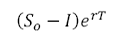
5. Forward Contract
a. Value of a long forward contract (continuous)
![]()
Where S0is the spot price
T is the remaining time to maturity
r is the risk free rate
K is the delivery price which is set in the contract
b. Value of a long forward contract (discrete)
![]()
c. Value of a long forward contract (continuous) which provides a known income
I is the present value at time 0 of the known income on the investment assets
d. Value of a long forward contract (continuous) which provides a known yield
q is the know yield rate provided by the investment asset
e. Value of a forward foreign current contract (continuous)
![]()
Where rf is the value of the foreign risk free interest rate when the money is invested for time T.
6. Forward exchange rates
![]()
Where r and rf are compounded continuously
or
![]()
if the interest rates were compounded on a discrete basis.
r is the risk free rate of the domestic currency
rf is the risk free rate of the foreign currency
Valuation of Interest Rate Swaps and Future Contracts
1. Interest Rate Swap
a. Net Cash Flow
The net cash flow for the buyer of the contract (receiver of floating leg and payer of fixed leg) at each payment date is:
![]()
Where t-1 is the payment date on which the floating rate interest was observed and is one payment date prior to the payment date on which the net cash flow is paid.
“days” are the period of time in the interest rate period (in years) based on the appropriate day count convention.
2. Futures
a. Stock Index Futures
These futures are used to offset the exposure to a well diversified equity portfolio, in particular the systemic risk associated with the portfolio.
The futures price of stock indices with known yield is as follows:
b. Futures Contracts on Currencies
The futures price is as follows:
![]()
Where F0 is the futures price in local currency of one unit of foreign currency
S0 is the current spot price in local currency of one unit of foreign currency
r is the domestic risk free rate
rf is the foreign risk free rate
c. Futures Contracts on Commodities
The futures price of a commodity with no storage cost or income is as follows:
![]()
The futures price of a commodity with storage cost and income is as follows:
![]()
Where U is the discounted value of the storage costs net of income during the life of the futures contract.
d. Futures Price for Treasury Bond futures contracts
![]()
Where I is the present value of the coupons during the life of the contract discounted at the risk free rate.
Financial Risk, Reward metrics and measures
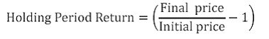
1. Holding Period Return
For the calculation of Sharpe and Treynor Ratio(see below) the holding period return derived above is scaled to a year, i.e. to 252 trading days if the holding period exceeds the number of trading days in a year.
2. Standard Deviation/ Volatility
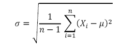
Where Xi is the ith price/rate and μ is the mean (average) of data set, i.e.
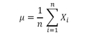 and ‘n’ represents the number of values in the data set.
3. Annualized Return
![]()
Where the number of trading days in a year = 252 days
4. Annualized Volatility
![]()
Where the number of trading days in a year = 252 days
5. Sharpe Ratio
![]()
Where RI is the Holding Period Return of investment I.If the number of days in the holding period exceeds the number of trading days in the year the holding period return is proportionately adjusted to arrive at the holding period return for a year.
Rf is the annualized risk free rate of return and ?I is the annualized standard deviation of rates of return of investment I.
6. Beta
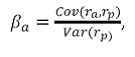
Where
ra measures the rate of return of the asset,
rp measures the rate of return of the portfolio of which the asset is a part, and
Cov(ra, rp) is the covariance between the rates of return.
In the Capital Asset Pricing Model(CAPM) formulation, the portfolio is the market portfolio that contains all risky assets, and so the rp terms in the formula are replaced by rm, the rate of return of the market. Rate of return of the broad market index is used as a proxy to the rate of return of the market
7. Treynor Ratio
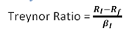
Where RI is the Holding Period Return of investment I. If the number of days in the holding period exceeds the number of trading days in the year the holding period return is proportionately adjusted to arrive at the holding period return for a year.
Rf is the annualized risk free rate of return. The risk free rate is the average rate on a risk free instrument during the period being analyzed.
βI is the beta of investment I with respect to a market benchmark. The market benchmark is usually taken as a broad market index.
8. Jenson’s Alpha
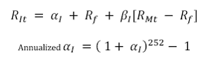
Where
αI = measure of the equity’s performance relative to the respective indices and represents the unique return of the investment.
RIt = The daily return of investment I at time t
Rf = The daily risk free rate of return = (1+annual risk free rate)1/252-1
RMt =The daily returns of the market index at time t
βI = The beta of the equities with respect to the market index
9. Correlation Coefficient, r
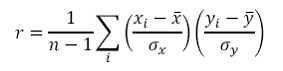
Where
n is the sample size
xi is the measurement for the ith observation of x
![]() is the mean of the observations of x
is the mean of the observations of x
σx is the standard deviation of the observations of x
yi is the measurement for the ith observation of y
![]() is the mean of the observations of y
is the mean of the observations of y
σy is the standard deviation of the observations of y
10. Portfolio volatility taking into account Correlations
![]()
Where

a, b and c are the weights of the respective asset in the portfolio X, Y, and Z are the assets in the portfolio
Variance(X) is the variance in the values of X, i.e. it is X’s volatility squared (σx2)
Variance(Y) is the variance in the values of Y, i.e. it is Y’s volatility squared (σy2)
Variance (Z) is the variance in the values of Z, i.e. it is Z’s volatility squared (σz2)
ρxy is the correlation between X and Y
ρyz is the correlation between Y and Z
ρxz is the correlation between X and Z
Black Formula’s, Valuing Interest Rate Caps and Floors
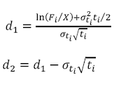
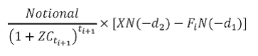
1. Black’s Formula
a. Value of a caplet
The value of a caplet which resets at time ti and payoffs at time ti+1 is:
Where
![]() is known as the forward premium
is known as the forward premium
X is the Strike
Fi is the forward rate at time 0 for the period between and ti+1
σti is the volatility of this forward interest rate
ZCt is the t- period spot rate / zero coupon rate and
N(.) is the cumulative probability distribution function (pdf) for a standardized normal distribution
b. Value of a floorlet
The value of a floorlet which resets at time ti and payoffs at time ti+1 is:
Where
![]() is the forward premium.
is the forward premium.
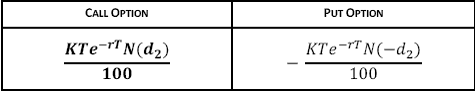
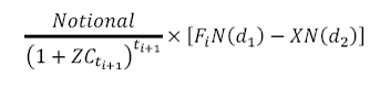
2. Value of a binary call option
The binary call option pays the Fixed rate * Notional if the interbank rate exceeds the cutoff rate. Its value is
![]()
Where N(d2) is the probability that the interbank rate will exceed the cutoff rate and
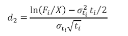
Where Fi is the forward value of the interbank rate, X is the cut off rate, σ is the volatility of Fi , zct is the t- period spot rate / zero coupon rate and ti is the time from the valuation date to time i.
3. Value of a binary put option
The binary put option pays the Fixed rate * Notional if the interbank rate is below the cutoff rate. Its value is
![]()