Earlier we had provided an overview to the Principal Component Analysis (PCA) process. In this post, we will consider the data that will be used in the analysis and the adjustments that would need to be made to the data before it can be used in the analysis.
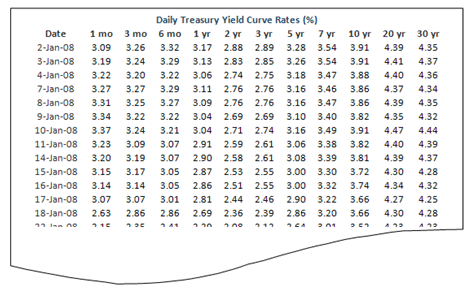
Obtain historical time series data

In a more generalized form, At time ti we observe rate, r(ti, τj) for j =1,…,k, where j represents the number of maturities in or dimensionality of the data. Again it should be noted that if we were conducting PCA to determine the volatility functions for a HJM interest rate model we would need the time series data for forward rates.
Select rate series for tenors to be considered
In our analysis we will be considering the following tenors:
- 3 months
- 6 months
- 1 year
- 2 years
- 3 years
- 5 years
- 7 years
- 10 years
Note that in Excel the Solver function has limited capability and will not work if too many tenors are included. If more sophisticated solving programs are not available and the reader has only to rely on Solver, he/she should select those tenors that would best describe the term structure of rates.
Removal of “jumps” in the data
As mentioned earlier the PCA process assumes that there are no jumps in the data. Therefore before proceeding any further with the analysis these jumps in the data have to be addressed. In our example however we have made no adjustments for any jumps that may exist in the data.
We have considered what data will be used in the PCA process and how the data will be adjusted. In the next post we will see how a covariance matrix of the differences between consecutive rates in a time series will be calculated.
If you would like to buy this course as a PDF file or the sample EXCEL sheets, please see the Interest Rate Modelling section at our online finance course store.

Comments are closed.