Variance Reduction tools for Monte Carlo Simulation.
Monte Carlo simulation techniques are a useful tool in finance for pricing options especially when there are a large number of sources of uncertainty (in modeling terms: state variables) involved. Unlike Black Scholes formula for which closed formed solutions usually do not exist when there are three or more state variables or numerical methods like binomial option pricing models which become impractical when the sources of uncertainty increase, Monte Carlo simulation techniques can lead to convergent solutions for these derivatives.
The solution’s accuracy however is dependent on the number of trials, N, that are used. Specifically the uncertainty surrounding a possible solution is inversely related to the square root of N. This relationship of accuracy to number of trials is derived as follows:
The mean of the discounted payoff, ?, is the average of the discounted value of payoff across all trials, i.e. the estimate of the value of the instrument. The standard deviation of these discounted payoff values is denoted by sigma or stdev.
The standard error of the estimate is given by sigma/root(N).
A 95% confidence interval around the estimate is given by:
mean-1.96*sigma/root(N) < estimate < mean+1.96*sigma/root(N)
This shows that as the value of N increases, the range around the estimate reduces, i.e. the accuracy of the estimate or the solution from the Monte Carlo methodology increases as the number of trials increase. Specifically, in order to increase the accuracy by a factor of x, the number of trials that should be used would need to be increased by a factor of x2. For example to double the accuracy of the estimate, the number of trials that should be used to ensure this level of accuracy would need to be quadrupled.
As the number of trials increases the Monte Carlo simulation technique becomes more and more time consuming as well as computationally intensive. In order to save on computational time there are a number of variance reduction techniques that may be used. These include:
- Antithetic Variable Technique
- Control Variate Technique
- Importance Sampling
- Stratified Sampling
- Moment Matching
- Quasi Random Sequences
We now present a simple illustration of two of the above techniques in increasing the pace of convergence using Monte Carlo Simulation techniques.
Variance reduction illustrated example
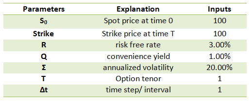
We consider a European call option on crude oil (WTI) where the current underlying spot price is 100; the strike price is 100. The annual risk free rate is 3%, the convenience yield is estimated at 1% and the annual volatility in the underlying price series is 20%. The option will expire in a year’s time.
Calculation models
Using the Black Scholes call option pricing formula we determine that the price of the European Call option. The Black Scholes solution for the value of a call option takes the following form:
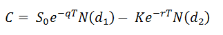
The value of the option using the closed form Black Scholes model is 8.827.
The form used for Monte Carlo Simulation based on the BSM framework works with the following equation
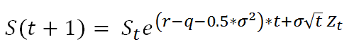
We now run the simulation for an increasing number of iterations and present the results from the original closed form solution and the Monte Carlo simulator below.

We see that the general trend is a reduction in the difference in values from the two approaches. Monte Carlo Simulation value converge towards Black Scholes Merton Model values as the number of iterations increase.
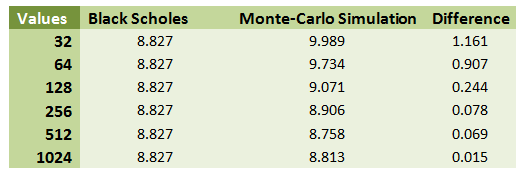
However increasing the number of simulation has a marginal impact on fine tuning of the value. A trend which is followed by all approaches and the trend lines in the error terms for each method suggests.
Next we look at the variation that the simulation provides. We call this variation the standard error term. We do this by calculating the standard deviation of the simulated results and divide them by the square root of the number of simulated runs.
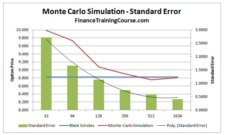
The chart shows that increasing simulation runs results in a decrease in standard error. This was indicated earlier as increasing runs resulted in convergence of Monte Carlo simulation value towards the Black Scholes Merton value.
Antithetic variable technique
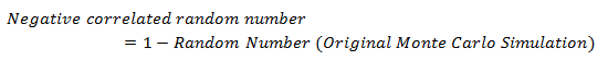
Antithetic Variable Technique uses two Monte Carlo simulations and takes the average. It doubles the sample size; it uses the original Monte Carlo simulation results along with its negatively correlated result.
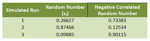
The random number for the negative correlated simulation is:
For example:
Putting the technique to work we once again plot the convergence between our revised Monte Carlo Simulation model and the original close form Black Scholes model price.
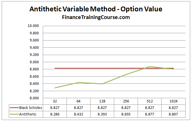
This average series of results converges towards the Black Scholes Merton value of the option at a faster rate via a different path than the results from the original Monte Carlo simulation.
Next is the standard error calculation. We calculate the standard deviation of the average series and divide it by the root of the number of simulated runs for a single sample.
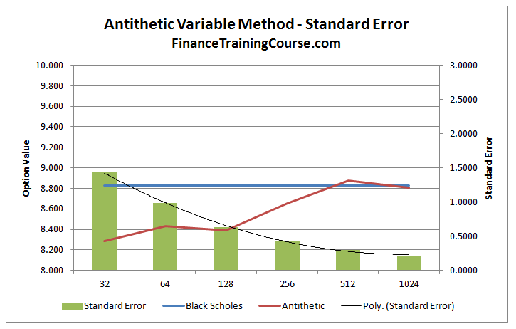
The comparison between the standard error terms above with the error terms from the original Monte Carlo simulation method shows a different and slightly shorter path to decrease in the error term.
Quasi-Random Monte Carlo Sequence
Now that we have the sequence, we calculate the simulated prices, intrinsic values and values of option for each simulated run as we have done before for Monte Carlo simulation. The results from the Quasi Random Monte Carlo method are depicted below:
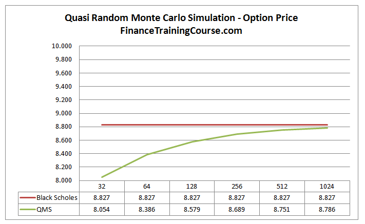
We can see that there is a significant improvement in the convergence rate of the results, in particular, in comparison with the original Monte Carlo simulation results.
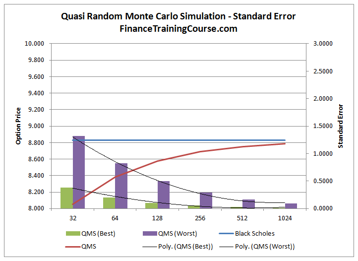
What about standard error under Quasi-Random Monte Carlo Simulation?
The data points drawn from the Quasi-random sequence for each simulated run are not independent of each other as is the case for the Monte Carlo simulation and the Antithetic method, but are selected to uniformly cover the entire sample space. Each subsequent number in the sequence is dependent upon the previous number. Because of this dependency, the standard error term cannot be calculated.
For a Quasi-random sequence method the best estimate for the standard error is the standard deviation of the sample divided by the number of simulated runs in that sample. The worst case or maximum error is the standard deviation of the sample times (ln(number of simulated runs)^dimension) divided by the number of simulated runs. The results are depicted in the graph below:
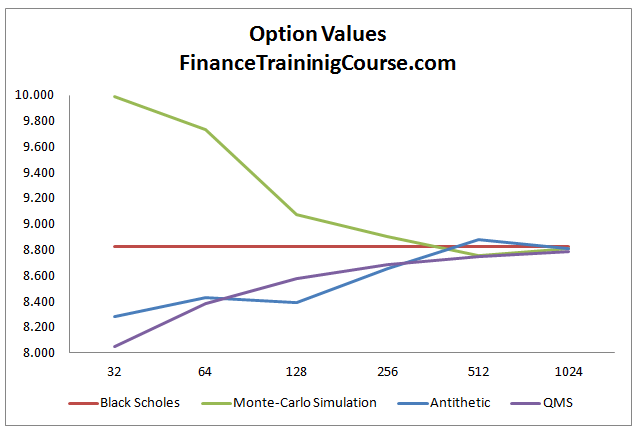
Note that we have purposely kept the axis scales for all the graphs the same so that you can see the extent of the improvement in results. To conclude let us see the results from all the methods together:
As is apparent in the graphs above, the results from the variance reduction procedures do in fact converge to the Black Scholes Merton value at a faster rate using a smaller number of simulated runs, different convergence paths and show much smaller deviations from the actual result as compared to the original Monte Carlo simulation method.
You are one smart guy.