FRM training lecture. MBA FRM Course, SP Jain Dubai, June 2012.
This is the actual transcript from the Shortfall session of my Financial Risk Management (FRM) course run at SP Jain, Dubai in June 2012. The language and tone is conversational and has been preserved as is. This was a two hour training session…
FRM Training Workshop: Correlation and Portfolio Volatility
What is correlation, and what is its formula? Please see the correlation page before proceeding further
Covariance between A and B divided by sigma A and sigma B. To find the variance of a portfolio, we use the following formula: sigma squared A plus sigma squared B plus 2 times A times B times sigma A times sigma B.
Let’s assume we have a portfolio of a 100 positions. How would the above formula expand in this case? Not very nicely, right? Therefore, to calculate the volatility of a portfolio, you create something called a variance covariance matrix. This is one way of working with portfolio volatility. What we will do is that rather than getting into the actual, detailed process of building a variance-covariance matrix which will become very cumbersome, we will use a shortcut. This shortcut will allow us to calculate the volatility of a portfolio using some of the tools and techniques that we have already used yesterday.
The first method, the variance-covariance matrix, is reliant on this assumption, which further needs portfolio volatility to work. As we saw yesterday, the shortfall with this method is that the (distribution of) asset prices in the actual world is not Normal. We do not have an appropriate name for what exactly it is, but we are sure that it is not Normal.
The second approach that you work with is called historical simulation. This is the same approach that we used yesterday when we built the histogram. In that, we looked at the distribution to count the number of points that we had for different price shock levels. Rather than guessing, we assumed that the underlying distribution was not Normal and looked at the true distribution instead.
The third and final approach is the Monte Carlo Simulation. To be fair, Monte Carlo is just a fancier extension of the first approach. The reason why I say this is because you need an estimate of volatility. Once you have that estimate, you use it to simulate a world which is Normal. So if I have a choice of using any one of these three methods, my preference as a practitioner is to always go with the historical simulation because it follows the true distribution. I will use Monte Carlo only when I have no related price data to work with to calculate historical returns.
One of the things that we will do today is to go through all three approaches quickly and build them so that we are clear in our mind over how different the results are with each specific approach. The second thing that we will do before you open your Excel sheets is to walk through a simple transaction where a customer has asked for advice on hedging his exposure. You as a banker/consultant have gone to see them. The example that we will be looking at will be for crude oil refineries.
Here are the client’s questions on hedging his risk exposure?
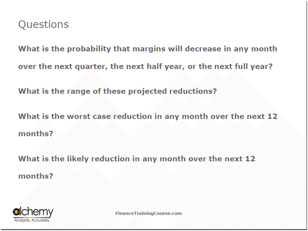
Figure 1 Risk Hedging questions – Client facing
FRM Training Workshop: Introducing Probability of Shortfall
One of the questions that you asked me was about calculating probabilities. You have all done microeconomics right? You understand the concept of breakeven analysis? Take this concept, but flip it.
The breakeven concept focuses on how much do we need to buy, sell or manufacture so that our costs are covered. Similar to breakeven is the concept of what we call shortfall, also known as in the insurance industry as the probability of ruin. The shortfall concept asks the same question but in a different way.
If, for instance, I have US $600 million in income, of which US $ 400 million are my expenses, I have a profit margin of US $ 200 million. The question that I am asking is about how much prices need to move for this margin to hit zero or even turn negative.
Yesterday, you calculated the volatility on a price series. Using this volatility, you applied it on a normal distribution to calculate what the price shock would be. The question that I am now trying to ask is what price shock would break either Air Canada or GM? Once I find out what that price shock is, then I need to find out the probability of that price shock occurring. This is a similar concept as breakeven analysis, but flipped on its head. Rather than focusing on how much do we need to cover our fixed costs, we are looking at how much do prices need to move for us to get into trouble.
FRM Training Workshop: Probability of Shortfall Crude Example – The Air Canada Fuel Hedging Case.
For example, I assume that a US $ 1 change in prices of the underlying commodity (whether it is Canadian Dollar, Fuel oil, WTI or gold) will lead to an added expense of US $ 30 million. Thus, prices need to move by about US $ 7 to add another US $ 210 million in expenses, while holding everything else constant. If I use this figure as the basis, then, all I need to figure out is the likelihood of prices moving by US $ 7.
Let’s also assume that the current price level is at US $ 3, and volatility is at 50% for a 12-month period.
If we (multiply) it by a (factor of) 3, we end up at 1.50, and if we multiply it by 5, we end with 2.5.This example is for Air Canada.
If prices move by US $ 7, the current price of the commodity would now be US $ 10. If I use 3, which corresponds to 99.9 percentile, at 50 % volatility, the factor would now become 1.5%, which is now the annualized volatility. 1.5 times 3 is a maximum shock of 4.5. Moreover, if I take a factor of 5 which corresponds to approximately 99.999 percentile, then 50% times 5 would be 2.5%. 2.5% times 3 would then be 7.5. So the question now becomes about the probability of getting multiplied by either of these corresponding percentile numbers? Subtract the corresponding NORMSINV numbers from 1 to calculate the probabilities.
Before we move on, did everybody follow what we just did?
Go through it step by step. What is the thesis of what we have done?
The thesis is that we want a model that allows us to estimate the probabilities that margins will decrease. If you take the extreme end, then we are figuring out the probability of the margin being zero or negative. My current numbers are that I make US $600 million in income, US $ 400 million in expenses, which leaves me with a margin for US $ 200 million.
The commodity that I have is fuel oil. The price series for fuel oil tells us that the standard deviation for a full year is at 50%. The current price is at US $ 3. In this specific case, I am assuming that for every dollar that fuel oil goes up, I will spend an additional US $ 30 million. If fuel oil goes up by a number greater than US $ 7 in the next 12 months, I will get to a point where I will spend an additional US $ 210 million in fuel costs. If I spend this amount, my margin will turn negative, and my net number, assuming everything else is held constant, will be US $ -10 million. The question that we are asking is what is the probability of this happening?
We go out and say that I have a very simple model which says that this is a distribution of changes in fuel oil prices. This model at the beginning has a standard deviation of 50% per year, which means 1 standard deviation move is 50%, 2 standard deviation move is 100%, and so on. For my margin to become negative, prices have to travel 5 standard deviations for me to end up with a margin of US $ -10 million. Although prices actually have to move by 7.5 as previously explained, for argument’s sake, we are assuming that they move by 5 standard deviations.
We are right now doing very basic work so that the fundamental principle is clear. Once this principle is clear, then we can extend it and get to the part of presenting this information to clients. The first tool in our toolkit is our shortfall method, and we have used it to estimate the probability that our margins will be negative. This is different from the probability that the price shock would be exceeded. Now that we have done piece for one specific scenario, there are more questions that we need to answer.
In this specific case, we made assumptions, such as that we had a profit of US $ 200 million, a dollar increase would lead to an increase in expenses by $30 million. Maybe this figure is not $30 million, but rather $60 or $50 million. If that is the case, then you do sensitivity on each of these elements, and you do analysis which is on a range of each of these elements.
We will now look into a simple case study of how we applied this to an oil refinery, and what were the drivers, the exposures, the sensitivities, and the final analysis.
FRM Training Workshop: Margin Shortfall Analysis – The Oil Refinery example and case
You are an oil refinery.
How does an oil refinery work? It buys crude oil.
How exactly does this process work? Let’s say you are an oil refinery in Tokyo, Japan. It takes around a 15 hour journey by air from where oil is to the oil refinery. Is it a good idea to transport oil by air? No. You therefore ship it, using a Very Large Crude Carrier (VLCC) . Let’s assume that a typical oil refinery in Japan buys crude oil in bulk anywhere between 50,000 to 100,000 tons. One ton of oil costs around $700-$900. Your supplier is ADNOC.
How long does it take a VLCC to go from Abu Dhabi to Tokyo? So think about this. I have bought 100,000 ton of crude oil. I have a ship near Abu Dhabi waiting for my confirmation. Once I give my confirmation, the ship first docks at Abu Dhabi, then loads and finally departs. The ship will not be docked and ready to load when I buy the oil. Let’s say it takes about three days for the ship to dock, load and depart. When the ship reaches Japan, it takes another three days to dock and unload. The oil is then transported via a pipeline from the port to the refinery, which makes it a total of 5 days until the oil finally gets to the refinery. This makes it a total of 8 days so far. What about the nautical distance between Abu Dhabi and Tokyo? Let’s make an assumption about this distance. Dubai to New York is about 7000 miles, lets assume Dubai to Tokyo is a similar distance. VLCC’S travel at a speed of 10 knots an hour, which takes around 30 days. In total, we are looking at a roughly 40 day window.
Now here is the challenge: if it takes around 40 days for crude oil to get to you before you can do anything with it, how long would it take you to refine that amount of crude oil? This depends on the capacity of the oil refinery in question. Let’s assume that it takes this refinery around 3 to 5 days to refine oil. You produce petrochemical products after refining crude oil. The biggest one of them is gasoline, followed by diesel, naphtha, and other derivative products. It takes another 3 to 5 days to you for getting these products in front of your customers. Thus, your end to end cycle, from the point that you purchase to the point of selling is around 55 to 60 days.
If the price of crude oil goes up, does the price of your petrochemical derivatives also go up by the same amount?
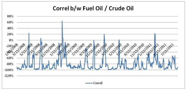
Figure 2 Correlation between Fuel Oil & Crude Oil
Here is the correlation.
Just like trailing volatility, we can also calculate trailing correlation.
In this case, it shows that the linkage between a petrochemical derivative product, which in this case is Fuel oil, and crude oil, is actually negative. There is no assurance of your prices going up if crude oil prices go up. So what has the refinery done? It has bought 100,000 tons of crude oil at $1000 per ton. This equals to US $100 million. For the next 60 days, it is not going to produce anything, and is exposed to this amount. At the end of the 60 days, it will know the relative price at which it can sell. Thus, its primary exposure is that if in those 60 days prices go up or come down, then what will happen? If the price of crude oil goes up once it has bought it, this inventory that it has in its books will go up in value. The products that are produced in those 60 days will also fully go up in value. If the inverse relationship holds, which is what we have seen, then if crude oil prices go up, the derivative prices will go down.
FRM Training Workshop. Oil Refinery Scenarios for estimating exposure
Think in terms of risks and exposures. You have around four/five things to worry about. Let’s make a list of all the things that can possibly go wrong.
1. Crude oil prices go up. Your $100 million also goes up.
2. Refined products, such as fuel oil and gasoline go down. You bought crude oil at a specific level, but will not be able to sell it at full price.
3. Crude oil prices go down, and refined prices also go down. Your inventory comes down in value, and the inventory that you are producing also comes down in value.
4. Nothing happens to crude oil prices and they stay the same. Refined products come down.
5. Crude oil prices as well as refined prices go nowhere. This is the best case since your costing does not change in this. In all the other cases, your costing takes a hit.
From a refinery’s point of view, there are two separate challenges.
The first challenge is that you have crude inventory that goes up and down in value. Since you do reporting on a quarterly basis, if you bought crude in the middle of the quarter, and right towards the end of the quarter crude oil prices fell, whereas your inventory is marked to the market, then what happens? Also, refineries are open for approximately ten months or 300 days and are closed for maintenance for two months. If it takes 60 days for end to end transit of one batch of crude oil, how many batches do you think are in transit at any given point in time? At least 50 days’ worth of batches are in transit at any point in time. This is around 5 million tons of crude oil. Thus, the refinery has an exposure to $500 million worth of crude oil which is effectively floating in the sea and will get marked to the market at the end of every quarter.
Is this good or bad?
Prices go up and down. For instance, you buy it at $80 a barrel, prices go up to $84 and come back to $80, which is fine. Even if they go down to $75,it’s fine. But if you bought it at $110 and prices come down to $80, that’s a 30% mark down. A 30% markdown on half a billion dollars amounts to a mark down of $150 million.
This is just the exposure from crude oil. What about the refined products?
If you are processing 100,000 tons a day, and you have the capacity to store another 100,000 tons, then how many days of storage would you have? So if you keep 30 days’ worth storage of refined products, you have 3 million tons of refined products. Thus, a total of 3 million tons of refined oil and 5 million tons of crude oil are open to the risk of prices coming down and being marked to market in your accounting statements at the end of every quarter.
Would you like to hedge this risk? If you were the CFO of the refinery, you would want to hedge this risk.
The question that you need to ask in all of these cases is how to figure out what part of this risk should be hedged. Let’s say that (we know) for both Air Canada and GM (the hedge ratio) is around 50% and 75%.
But why? To do this, you need to take a step back. Go look at the process and apply the calculations for the shortfall. Apply the same analysis to figure out how much would these price changes bring on hits in the P&L.
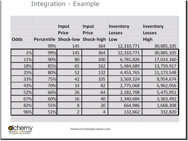
Figure 3 Applying Shortfall to Crude Oil Inventory Losses
Here is the range of percentiles from 99 to 51 percentiles.
We figured out two price shocks corresponding to each of these percentiles. There is a stable vol (volatility) world, in which volatility is at the lower end, and then there is a high vol world, in which volatility is at its peak. Let’s do our analysis on both.
We then figured out the dollar magnitude in inventory losses in a given period across both, the high vol as well as the stable vol world. The question that we put to the board in this specific case was that when I say 51 percentile, the odds are almost even. There is a 1-1 chance.
You should see this change almost every other day. We then asked them about the most common change that they see because that would give us an idea about how to calibrate what we have in front of us with the market that they operate in. They said that the most common change that they saw was a change of $27. This $27 relates to 66 percentile. Now, the odds are one chance of happening, and two chances of not happening. The loss that corresponds to this level is around $2 million per quarter in the low vol world, and $7 million per quarter in the high vol world. Incidentally, this is a small refinery, and therefore the tonnage that they have is not very high.
How do you make a decision on the basis of these numbers? The question that you should ask to yourself is that if you are a member of the Board of this refinery, are you comfortable with seeing a direct hit to your P&L because of mark to market losses of about $7 million at least six to eight times in a given month?
We had created a grade and asked the board to pick a grade that they were comfortable with. The board came back and said that they could do with a loss of US$ 3 million, but anything above it did not make sense. This $3 million now becomes a threshold.
In the GM case, when you’re saying that you are covering 50% or 75%, you are effectively saying that you are okay with taking half the exposure on ourselves, and only covering the remaining half.
You all have health insurance in Dubai right? Somewhere in the language of your health insurance forms, it says that expenses up to a certain level will not be covered, and beyond it will be covered. That is called a deductible. Same thing is applied to your automobile insurance back home in India.
In this case, the deductible set by the board is $3 million and the level of coverage that you want to buy starts above a price shock of $16 per ton in the low vol world and $40 per ton in the high vol world. Thus, the protection that you want will only kick in once prices have risen above these price shocks.
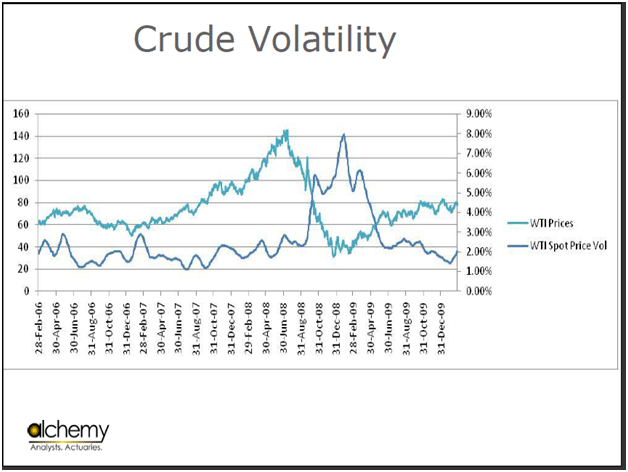
Figure 4 Crude Oil trailing volatility and price changes
If you now look at crude volatility as shown in this graph, you can actually see that crude goes all the way up till 8% in terms of volatility and comes down to 2%. This data is from 2006-2009. However, is our analysis enough, or should more be included in it?
Financial Risk Management Training: Oil Refinery & Crude Oil changes. Challenges
Let’s look at this. Your primary issue is exposure in terms of the lag between purchase and product arrival for distribution. If you are regulated, then your retail price is sensitive to the price set by the market regulator, which in most cases is the Oil and Gas Regulating Authority. The market regulator links market price to the international crude price, which may be completely different from the lag that you are facing in terms of purchase and delivery. Then there is a 30 day lag in every price reset. This makes it even more interesting. When you buy crude from ADNOC, how do you think pricing works?
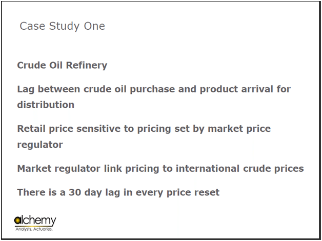
Figure 5 Oil refinery lag challenges.
Today is the 3rd of the month. I am now buying a 100,000 ton batch every day for the next 30 days. When I buy the batch do I know what the price is? The actual cost of what you have bought will be determined and set at the end of the month. Thus, there is also price uncertainty at the time of purchase, which means that I do not know the price at which I have bought the crude. It is a function of what happens to prices in that month. My pricing will be locked in only at the end of the month when ADNOC comes out and says that pricing for the batches sold for the month of June is X amount of dollars.
There are different suppliers who have different pricing mechanisms in place. For a second, let us assume that you have uncertainty on both sides.
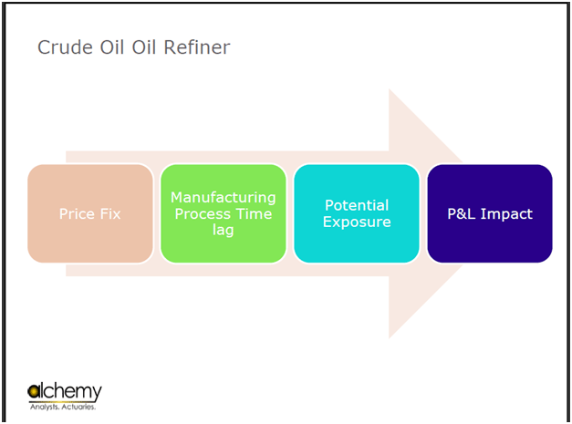
Figure 6 Oil Refinery hedging case. From price fix to P&L
If you review the process that we have gone through, there has been the Price Fix, the Manufacturing Process Time, Potential Exposure and finally the P&L impact of that exposure.
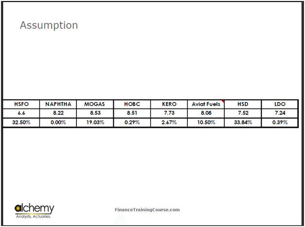
Figure 7 Oil Refinery – Refinery Yield Mix
The assumption is that the refinery that we are working with produces high sulfur fuel oil (HSFO), naphtha, gasoline (MOGAS), high octane (HOBC), kerosene (KERO), aviation fuels, high speed diesel (HSD) and low speed diesel (LDO).
Each barrel of oil that the refinery uses produces about 32% in high sulfur fuel oil, 19% in motor gas, 0.29% in high octane, 2.6% in kerosene, 10% in aviation fuels, and 33% in high speed diesels. This is relevant because you are now getting to refined products. In the first part we only looked at crude. Now, we need to look at the relationship between crude and refined products to calculate their exposure.
Financial Risk Management Workshop: Crude Oil Refinery Case: Putting the Exposure Estimation Framework to work
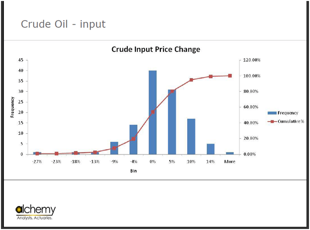
Figure 8 Crude Oil price change per ton per month – 5 year history
We then look at the range of price changes. For the period in question here, the range is -27% to +14%. The data is skewed. This was the input price change.
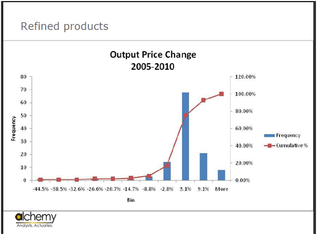
Figure 9 Impact of crude oil price change on petrochemical output prices
Now lets look at the output price change, which is -44% to +10%. Is it Normal? Finally, look at the Margin Change.
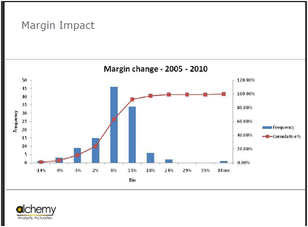
Figure 10 Impact of crude oil price change on Refinery margins
The first table only focused on crude.
This table shows that if you look at historical changes in margin over a time frame, you are looking at margin impacts of about -14% to +35% in an un-hedged world. Despite all of the volatility over the past five years, the net impact of all of these changes is still -14%. That is your exposure. How does that translate into numbers? The first graph that you saw showed you crude oil changes.
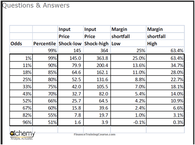
Figure 11 Crude Oil Refinery – Margin Impact of oil price changes
This shows things a little differently. It shows Input Price Shock-High & Low and the impact of the Input Price Shock on Margin Shortfall. It shows the amount by which margins change due to price shocks. Your worst case scenario is a reduction of 63%, and your best case scenario is that there is no reduction in the margin.
Financial Risk Management Case: Oil Refinery Hedging Case: Conclusions
Now, the Board has two different questions. The first is about how much do they want to lose in inventory loses. The second question is the percentage of reduction in their P&L that they are comfortable with. If my margins reduce by 22%, then things start getting a little uncomfortable. This corresponds to a threshold of 80%. From a protection point of view I have two dimensions now. The first dimension is crude oil prices and my inventory loss due to those prices. The second is that if I translate that loss into margin impact, I am looking at a margin reduction of 22%. From a policy point of view, I want a solution that would restrict the changes in my profitability to above 22% on account of an input price shock. That is the solution that I want. How do you create this? Will it be enough to just buy a forward contract on crude oil? You have figured out how much the board can lose, i.e. 22%. How do you structure this protection? If you were to buy a product for protection, that product would be linked to WTI and Brent.
You don’t have a product that gives you protection against oil bought from Abu Dhabi. What do you do? Think about based on what I have just shared, how would you move forward with the two cases, Air Canada and GM.
Comments are closed.