In this post, we model a fixed income portfolio by optimizing the allocation across the universe of securities using duration, convexity and EXCEL solver.
It doesn’t matter if you manage a pension fund, a life insurance trust fund or the proprietary book of an investment bank, at some point in time you hit your allocation and risk limits and need to rebalance your portfolio.
In most instances, your limits and target accounts focus on interest rate sensitivity, volatility, Yield to risk ratios, liquidity and concentration limits. Your objective is to create the most efficient fixed income investment portfolio that balances an optimal mix of the above constraints against yield to maturity. The time tested, the risk versus reward tweak.
In our new risk training workshop for fixed income portfolios case study, we will build a simple model using Excel solver that shows how to handle the fixed income portfolio optimization problem. We can easily extend the model to handle larger portfolios and additional constraints around liquidity, factor sensitivity, volume concentration, value at risk and volatility.
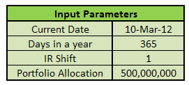
For the purpose of this case study, we will assume that we are advising a large pension fund who is re-evaluating fixed income portfolio allocation due to its new investment policy. The assets under management at the fund are US$500 million. We want to recommend:
- Portfolio allocation that minimizes duration
- Portfolio allocation that maximizes convexity
The liabilities are also equal to $500 million with a weighted average maturity of 20 years. Modified duration or interest rate sensitivity of liabilities was last measured in the monthly risk report at 9%.
Introducing Duration and Convexity
Duration is a measure of how prices of interest sensitive securities change as the underlying rate of interest changes. For example, if the duration of a security works out to 2 this means roughly that for a 1% increase in interest rates price of the instrument will decrease by 2%. Similarly, if interest rates were to decrease by 1% the price of the security would rise by 2%.
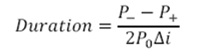
Here is the numerical approximation for modified duration.
Convexity
The Duration approximation of a change in price due to changes in the yield works only for small changes. For larger changes, there will be a significant error term between the actual price change and that estimated change using duration.
Convexity improves on this approximation by taking into account the curvature of the price/ yield relationship as well as the direction of the change in yield. By doing so it explains the change in price that is not explained by Duration.
A positive convexity measure indicates a greater price increase when interest rates fall by a given percentage relative to the price decline if interest rates were to rise by that same percentage. A negative convexity measure indicates that the price decline will be greater than the price gain for the same percentage change in yield.
We use Duration and Convexity together to immunize a portfolio of assets and liability against interest rate shock.
Introducing the Optimization model
Our first scenario assumes a rising interest rate outlook. Ignoring liabilities and maturity mismatch for now, our fund manager would like to rebalance the portfolio to minimize duration so that the value of assets does not fall significantly due to changes in interest rates. We assume:
Fixed Income Investment Portfolio Management: Breaking down the optimization model
There are four parts to this model:
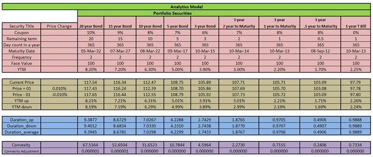
Part 1- The securities universe specification
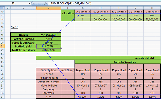
This is the pink-shaded area and defines the complete investment universe. You can only allocate a security that is present in the universe. Assets are classified in buckets of 20, 15, 10, 5 and 3 year maturities. We have assumed that the current date (the valuation date) is the same as the date of purchase (the settlement or value date) for all assets in all buckets.
Part 2 – The securities pricing model
The area in brown calculates the price and yield. We calculate Current Price using the EXCEL price function as illustrated below:
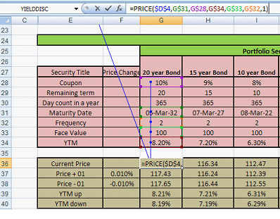
The EXCEL price (bond pricing) function is based on the data inputs of settlement date, date of maturity, coupon rate, yield to maturity, frequency and basis. Frequency here is 2 which means the semi-annual payment of coupons. Cell $D$4 in the input parameters refers to the current date.
We calculate price changes (Price + 01 & Price – 01) by adding or subtracting the specified interest rate shocks and recalculating new prices for use in duration and convexity calculations. The rate shocks are 1 basis points (1/10,000).
Part 3 – Portfolio Duration Calculation
The area in blue shows duration calculations. We calculate Duration using the duration approximation formula introduced above, which we present here again:

In the context of the Analytics Model, we calculate it as follows:
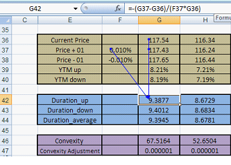
In the calculation of Duration-down, Cell G44 is replaced by G45 and F44 is replaced by F45. Note that the general form of the formula is applied but instead of just calculating duration in one line, duration up and down are calculated respectively and the average of both is taken. This average of the two durations will be used in our model.
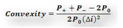
Part 4 – Portfolio Convexity Calculation
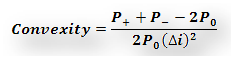
The final part of the model calculates convexity and is highlighted in purple. The applicable convexity formula is:
The calculation is as under:
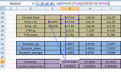
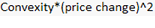
The convexity adjustment is calculated using the formula:
Fixed Income Investment Portfolio Management: Summarized Portfolio Analytics
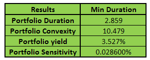
We now need a summarized portfolio analytics table that can be used in our optimization process. The results derived by combining the actual portfolio allocation and the portfolio analytics generated above would appear as shown below:
How can we calculate these results? The answer is through the Analytics Model and the allocation of assets followed currently for each bucket. The allocation table is shown below:

Notice that the total bond portfolio allocation is 97% and not 100%. Cash and/or non-interest sensitive securities make up 3% of the allocation.
Portfolio Duration
We calculate Portfolio Duration by using the EXCEL sum-product function.
Sum-product is simply the combination of two operations that involves multiplying the individual cells in two vectors (Portfolio Allocation, Security Duration) and then summing the resulting product across all cells.
For instance (10%*duration average for 15 year bond) + (10%*duration average for 10 year bond)….. And so on.
Portfolio Convexity
We calculate Portfolio Convexity in the same manner by using the EXCEL sum-product function. (10%*convexity for 15 year bond) + (10%*convexity for 10 year bond)….. And so on.
Portfolio Yield
And ditto for portfolio yield calculations. (10%*portfolio yield for 15 year bond) + (10%*portfolio yield for 10 year bond)….. And so on.
Portfolio Sensitivity
We calculate Portfolio sensitivity of -0.028600% in the following way:
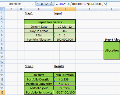
IR shift is the interest rate shift in basis points.
Portfolio Optimization using solver
If we had a single linear equation representing a single constraint and a single position, the Excel Goal seek function would be sufficient. However, a multi position fixed income investment portfolio has many constraints and many positions. In addition, because you are dealing with bonds, the underlying model is no longer linear. You need a non-linear tweak to make it work.
The Excel solver function helps us optimize our portfolio allocation model with a few tweaks. We demonstrate the simplest of scenarios in this write up but we can very easily extend them. As is the case with all optimization models, the trick is in designing the constraints. While there can be only one objective function (minimize or maximize a specific portfolio metric), with the right constraint design you could get close to a near optimal solution reasonably quickly. While the current model focuses only on fixed income investment portfolio, we can also extend the design of the model to include multi-class portfolios. In addition, we can add new target accounts and risk constraints just as easily.
Optimizing the base case – Minimizing duration
The trustees of our pension fund have given a target to the investment fund manager to earn at least 3%. The bond proportion should be 99% of the fund, with the remaining for cash. Risk management and diversification targets specify allocation of no greater than 13% of the total fund in any given asset bucket.
Given these objectives, how should the investment manager set out to minimize duration?
The targets are effectively constraints. Once we have defined them correctly, the solver function takes these constraints into account, evaluates the target optimization cell (minimize duration), and searches for an optimal solution. Since the layout of the spreadsheet has been described above, all we know need to do is to define the solver model and click solve.
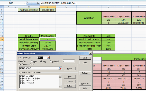
Pick ‘Min’ as your objective and then click ‘Solve’. Solver will work through the model until it reaches the optimal solution. The revised fixed income portfolio allocation is as follows:
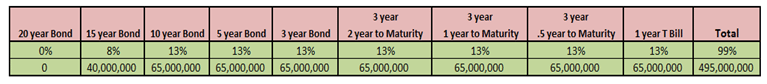
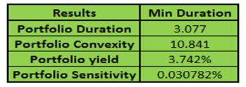
Note that none of the asset buckets have a higher than 13% proportion of assets. Also, bonds account for 99% of the investment, the rest is in cash. The revised portfolio analytics table summarizing our target account is below:
Maximizing Convexity
Positive convexity is generally a desirable attribute in a portfolio. In addition to minimizing the duration, an alternate case could be made for maximizing convexity. If you expect rates to decline, a more convex fixed rate asset would rise by more compared to a less convex asset.
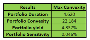
All it will take is to set the Target Cell as the portfolio convexity instead of duration. Note that in solver we click on ‘max’ instead of ‘min’ this time. The revised allocation is as follows:

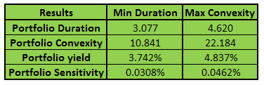
And the revised portfolio analytics results for both the maximized convexity and minimized duration scenarios are presented below:
Fixed Income Investments Portfolio Optimization. Next steps
You can easily extend the model to include constraints for value at risk, volatility, interest rate mismatch, gap management, concentration, portfolio liquidity, daily, monthly and weekly turnover, credit ratings and grades.
Also see: An alternate approach for calculating Economic Capital using accounting data rather than the BIS guidelines using the difference between Expected and Unexpected Loss.
Like this post – check out the new book – Portfolio Optimization Models in Excel, Revised Edition – Excel templates and dataset included.
Comments are closed.