The investment management function for a life insurance company faces multiple challenges. We try and address some of these challenges as part of the final problem set for the portfolio management course. The objective is to come up with the optimal investment allocation percentages for a life insurance company investment portfolio after testing multiple allocation strategies.
Insurance investment portfolio management
Like a bank, a life insurance balance sheet borrows money from policyholders for long durations and invests the proceeds in long term assets. Unlike a bank, a life insurance company is able to protect itself from unplanned short term withdrawal by levying what are termed as surrender and pre-mature liquidation charges. This provides an incentive to change the investment horizon by reducing the required liquidity profile.
A life insurance company provides a service. The service is the provision of financial protection to policyholders against unexpected death or disability. For this service, a premium is charged that covers the cost of protection in the short term and has sufficient margin built in so that the amount paid every year grows into a tangible pool of savings over the life of the policy. So the service is essentially intermediate protection while the savings pool created for the benefit of the policyholder grows to a level where it can provide the promised protection.
By design, long term liabilities backing life insurance products require an invest policy that gives higher weightage to safe, less volatile and long term assets. At the same time, the threat of inflation requires them to seek at least some exposure to inflation hedges. Within the investment universe, equity markets provide the strongest candidates for inflation hedges. Third, the nature of interest rate mismatch combined with the leverage in the balance sheet requires them to manage their Asset Liability Management exposure within narrow bands. This band is determined by the amount of fluctuation allowed by the investment policy in the original surplus (assets – liabilities) of the policyholder investment fund.
These challenges result in interesting portfolio management and optimization problem. We try and address that challenge in this post.

From a design perspective we need to do the following:
Measure duration and convexity for both assets and liabilities and then match them so that the difference between them is immunized to changes in the interest rate environment. This is one layer of our problem. We use the duration and convexity calculator to estimate duration and convexity of the bonds in our portfolio. We have been provided estimates for both metrics on the liabilities side.
The two equations for surplus immunization are:
Weighted average duration of assets = weighted average duration of liabilities
Convexity of assets > convexity of liabilities
For the inflation hedge – we need to test a number of different security and allocation combination. Our investment policy statement sets some guidelines on how much non fixed income exposure we can take. We play with that range to see how much spiced up return can we add by taking on other asset classes.
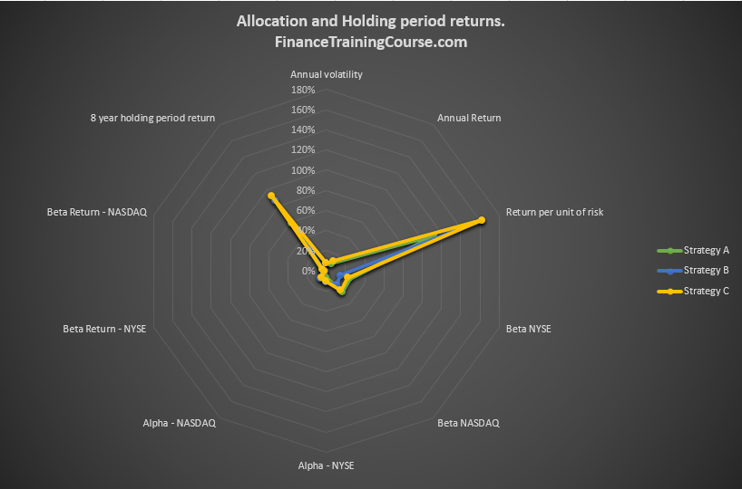
Our final test is that of Alpha. Can the double Beta strategy work in this scenario also? How does the strategy perform across shorter time horizons as well as longer ones? What happens to holding period returns for the alternate allocations when we run them through our evaluation period? We are also interested in finding out that on a alpha per unit of risk basis which asset classes provide the biggest pickup – equities, commodities or currencies?
Building up the spreadsheet – Insurance Investment Management
Let’s begin. Here is the high level sequence of events you would need to perform to complete the challenge. Go ahead and do this before we post the solution in the next 24 hours. (Ps – if you have just joined us and need the data set for the problem or need to get to the final spreadsheet see the Portfolio Management course post)
Step 1 – Measuring Duration and Convexity for assets in our portfolio
We use the duration calculator to get duration and convexity estimates for our portfolio. They are?
Step 2 – Modifying the spreadsheet
We plug the numbers into the investment allocation sheet and also estimate portfolio duration and convexity. We have been given duration and convexity estimates for our liability portfolio.
Step 3 – Updating the Solver model
First order of the day is to match duration and convexity for the two sides using between 90 – 85% of the allocation space. We have now managed to immunize our portfolio against interest rate changes. Changes in liabilities values will be more or less offset by changes in asset values. That is what we expect the model to do.
Step 4 – Finding the perfect non fixed income allocation
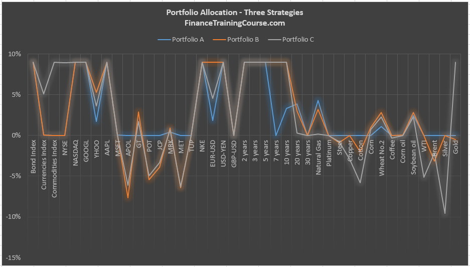
Our next challenge is that while keeping the same allocation in place, can we pick non fixed income assets that can add both yield and reduce portfolio volatility.
We have a few options. Option 1 is built without taking into consideration Alpha and Beta.
Option 2 is built with taking into consideration our standard rule – Alpha > Double Beta return. Given our preference for both stability and reducing price fluctuations, we use a different metric this time – Alpha/unit of risk to optimize our Alpha allocation.
Step 5 – Evaluation
How do the two portfolios perform? How is Alpha different from convexity? Use the same evaluation framework presented earlier in the course using holding period returns for the two portfolios across both the construction period and an evaluation period.