Value at Risk – Calculating Portfolio VaR for multiple securities with & without VCV Matrix .
In an earlier VCV Matrix post we had presented the theoretical proof of how the portfolio VaR obtained using the short cut weighted average return method produces the same result as would have been obtained if a detailed Variance Covariance matrix derivation approach had been used. In this post we look at a specific example where daily VaR for the sample portfolio is first obtained using the short cut technique and then the same result is arrived at using the detailed matrix methodology.
The portfolio is assumed to consist of two equity instruments, two FX forward instruments and two bonds. The returns series have already been obtained from the historical series of prices for all securities (including bond prices).
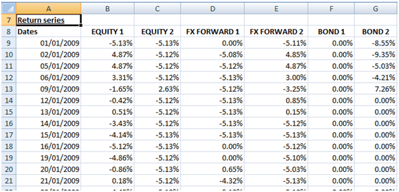
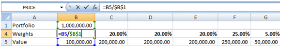
We have also determined the weights of each instrument as the value of each instrument in the portfolio to the total portfolio value. Please note that in our illustrations these values have been taken as given.
Calculating Value at Risk without VCV Matrix.
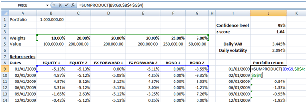
Using the short cut technique we derive a weighted average return series for the portfolio. In EXCEL the portfolio weighted average return is determined for each date as SUMPRODUCT (Array of returns for that date, array of instrument weights).
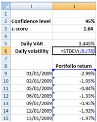
The daily volatility for the portfolio then equals STDEV(Array of portfolio returns). Note that in EXCEL the STDEV formula is calculated as 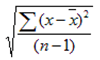 using the ”n-1 method (as sample mean, x_bar, is being calculated from the data), where n is the sample size (=70 in our illustration):
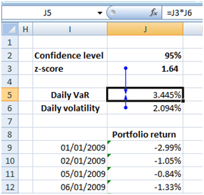
The daily VaR of the portfolio is Daily Volatility times
the z-value of standard normal cumulative distribution corresponding with a specified confidence level. Using a 95% confidence level the z-score =1.64. The resulting daily VaR is 3.445%.
Value at Risk using VCV MATRIX
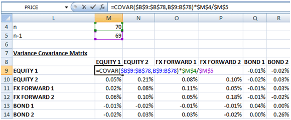
For the detailed VCV matrix method we need to first define a six by six (based on the number of instruments in the portfolio) variance covariance matrix as shown below:
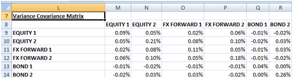
Each element in the grid is a covariance between the returns of the instruments in the intersecting row and column. For example cell M10 is the covariance between the returns of Equity 2 and Equity 1. The covariance between the returns of an instrument with the returns of itself is by definition the variance. In EXCEL however there will be a difference between COVAR (Array of returns of Equity1, Array of returns of Equity1) and VAR (Array of returns of Equity1) (VAR as in variance). This is because the former is calculated using the ‘n’ method while the latter is calculated using the ‘n-1’ method:
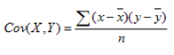
VAR (X) =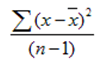
As the short cut method uses the function STDEV for calculating the portfolio’s daily volatility which also employs the ‘n-1’ method, EXCEL’s COVAR function has to be adjusted by multiplying it with a factor of [n/(n-1)] to make it consistent with the STDEV() function. Hence covariance elements in the matrix grid are calculated as given below:
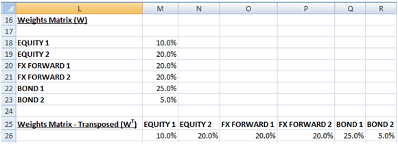
The next step is to present the weights of the instruments calculated earlier in two ways. A six by one vertical matrix, W, and its one by six transpose, WT.
Daily volatility is then determined in three stages as follows using EXCEL’s matrix multiplication function, MMULT (), and square root function, SQRT ():
Stage 1: Matrix 1 = MMULT (Variance Covariance Matrix, W)
Stage 2: Matrix 2 = MMULT (WT, Matrix 1)
Stage 3: Daily Volatility = SQRT (Matrix 2)
Putting all three stages together we have daily volatility determined as in the screen shot below:
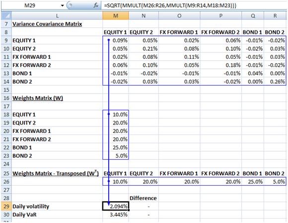
As you can see the result is the same as calculated earlier using the short cut technique. Daily VaR is is calculated as mentioned before, i.e. Daily volatility times z-score corresponding to the confidence level = 2.094%*1.64 =3.445%.
Value at Risk using VCV MATRIX – Using Correlations
As mentioned in the post:
another way of calculating the VCV matrix that will not require you to make the adjustment for the difference in EXCEL methods for COVAR and VAR (STDEV) is to first calculate CORREL (Excel’s correlation function):
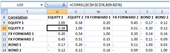
and then multiple the resulting number with the STDEV()s of the corresponding instruments in the intersecting row and column of the matrix grid to arrive at covariance. STDEV (array of returns of a given instrument) is the daily volatility of the instrument determined from its return time series:
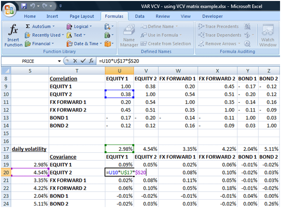
You can see that this grid is similar to the VCV matrix determined earlier. The added benefit, though, is that we now have the grid of correlations which we can utilize to give us further insights. Correlations may be changed to see the impact on VaR numbers. Note implicit in this manipulation of the correlation matrix though is that the underlying series of returns and volatilities as well as the correlations of those instruments with others in the portfolio remain unchanged. This is counterintuitive as CORRELs and volatilities are determined from the same returns series. However, despite these limitations useful insights may still be obtained and the methodology may be used for stress testing the portfolio.
For example, what is the impact on the VaR number if the all instruments were to become perfectly correlated with each other due to certain market conditions?
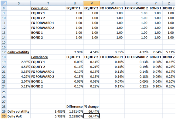
The portfolio daily VaR increases from 3.445% to 5.733% under this stressed condition – an increase of more than 66%.