While we introduced the concept of implied and local volatilities in lesson one on volatility surfaces we didn’t spend time in differentiating between the two volatilities. In our third lesson, we try and shed some (not a lot) light on a topic that causes confusion, heartache and pain in students of volatility surfaces. What is the difference between implied and local volatility
Implied volatilities
An implied volatility estimate is essentially a reverse solution for the value of sigma (volatility) given a price for a call or put option using the Black Scholes equation. A generalized treatment assumes the same value of implied volatility using the Black Scholes equation for all strike prices (K) and expiries (T) for a given underlying security.
More importantly, it is a price quoting convention that allows market participants to communicate their assessment and expectations with respect to expected future realized volatility. By definition as well as design it is not a model pricing parameter.
In lesson two when we spoke about the impact of rising volatility on deep out of money options and showed a range of option prices across different strikes, they all used a single implied volatility estimate. The problem with this single volatility assumption is that such a model cannot accommodate documented volatility smiles and skews.
Local volatilities
A local volatility model calculates volatilities for different combination of strike prices (K) and expiries (T). It does this in a market consistent no arbitrage manner. In simple English, this means that for a given date, time, underlying spot price combination, local volatilities are calculated in such a fashion that the resultant option prices match market prices. This assumes that we treat market prices as correct and arbitrage free and wish to calibrate our volatility model using basic liquid securities. Such a calibrated model (using basic securities) can then be used to “correctly” price illiquid exotic derivatives. A volatility surface represents such a generalized calibrated model. It creates a surface that makes it possible to generalize a “local” volatility value for all combinations of strike prices and expiries, something a simplified implied volatility model cannot deliver.
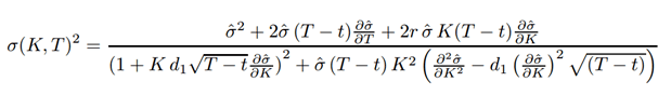
Derman and Kani trees and Dupire’s formula are two approaches that we commonly see in this space. Dupire’s formula (see below) is the approach that we introduced in building volatility surfaces and the approach we will use in following lessons to produce our volatility surface.
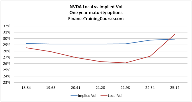
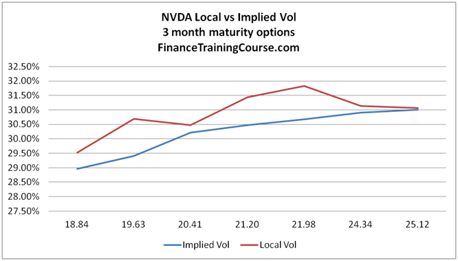
And now for a visual summary in English that is easier to understand for ordinary mortals. Sometimes a picture is worth a thousand words. In this instance, four pictures are worth four thousand words. The first three images plot implied volatilities and local volatilities for 3 year, 2 year and 3 months NVIDIA call options respectively for a given date, spot and time to maturity. The two variables in each of the plots are vols and strike prices.
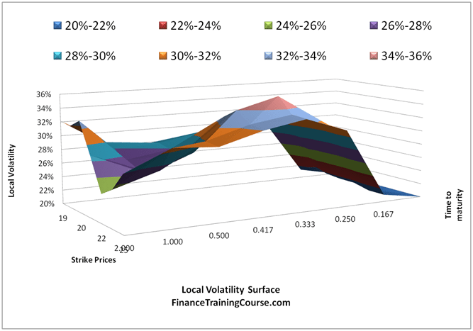
The three plots show three different relationships between implied and local volatilities. The three relationships are only a small sample of the options universe on NVIDIA shares. The fourth shows the completed volatility surface for NVIDIA incorporating the universe of these relationships.
If you are still reeling, here is a hint. Market consistent. Arbitrage free. Think about it till we return with our next lesson.
And now without further ado we present the four pictures.

Comments are closed.