This is our first post in a multipart series on volatility surfaces, their construction and usage in the option pricing world.
The source of implied volatility data is ivolatilty.com, an exceedingly convenient and cheap tool for downloading implied volatility and volatility surface building datasets. Tickers used in examples below and later posts include Barclays Bank (BARC:L), Nvidia (NVIDA), Tupperware (TUP) and Merck (MRK) pharmaceuticals. Equities that we (the authors) tend to follow as investors.
The many flavors of volatility
In the option pricing world volatility comes in many flavors. When you first download the price series for an underlying security and calculate the daily returns for the entire review period, the volatility estimate you generate is called empirical or historical volatility. It gives you an indication of how much prices have moved in the historical period you have just analyzed and are likely to move if history was to repeat itself. If your review period is 5 years, a 5 year average volatility estimate is really not going to help you price a 90 day option or estimate the price risk associated with the underlying security. On the other hand, if you are looking for a distribution of volatility to get an indication of the range volatility is likely to follow, trailing volatility, a moving average of volatility is a great tool.
However, the problem with trailing volatility is that it still relies on historical or empirical data. What we really need is a market consistent estimate of volatility that can be used to match (calibrate) market based option prices. Enter implied volatility. Pick an option, use its currently quoted price, plug in the Black Scholes equation and solve for the value of volatility that would lead to that price. At any given point in time historical volatility is our best estimate of what happened in the past. Implied volatility is our estimate of the level of volatility at which a market participant is willing to trade (buy or sell) his position. If historical volatility levels are higher than average they are likely to revert to the mean. As a trader, I would rather sell than buy options at this level. If volatility levels are at historic lows, they are likely to rise higher. Once again as a trader I would rather buy options than sell at these levels.
The challenge here is that implied volatility levels change based on the moneyness of options in question. For a simple call option on one of our above tickers, the implied volatility level move up and down depending on how in or out of money our call option is. For example Figures 1 and 2 below show plots of implied volatilities by moneyness for MRK and NVDA options that will expire in 30 days. The plot, given its shape, is popularly known as the volatility smile.

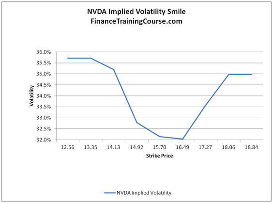
If you were a novice or naive option trader, unaware of the smile and you used implied volatility levels inferred by at the money options to price your out of money positions, your active option trader status will not survive beyond a few trades.
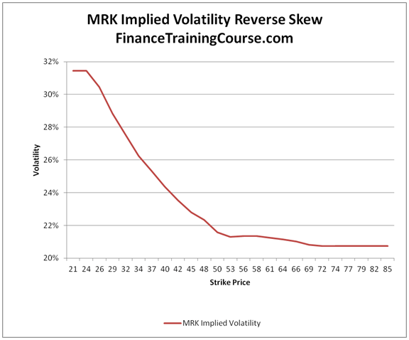
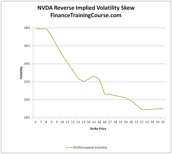
However, volatility smile is not the only twist in this game. If we shift our focus from 30 day options to longer 36 month options, we get a somewhat different shape when we plot implied volatilities for MRK and NVDA. In both images, we see that implied volatilities for lower strike prices (call options) are higher when compared with implied volatilities for higher strike prices.
Enter volatility surface
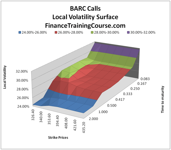
A crude conclusion after reviewing the four images above is that if you decide to model market consistent implied volatility behavior, you would need to factor in moneyness (strike prices) as well as maturity (expiry). Enter volatility surface.
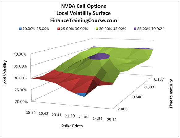
A volatility surface plots market consistent volatilities across moneyness (Strike prices) and maturity (time to expiry). Within the surface market consistent volatilities are referred to as local volatilities. Rather than backing out volatility by applying the Black Scholes model in reverse to at the money options, local volatilities use implied volatilities and a one factor Black Scholes model to drive local volatility values across the surface.
The end result when applied to the entire universe of Barclays Call options is something along the lines of Figure 5. Or with NVIDIA call options in Figure 6.
Klaus Schmitz quotes Ricardo Rebanato (1999) in his PhD Thesis at Oxford college.
“Implied volatility is the wrong number to put into wrong formulae to obtain the correct price. Local volatility, on the other hand, has the distinct advantage of being logically consistent. It is a volatility function which produces, via the Black-Scholes equation, prices which agree with those of the exchange traded options”.
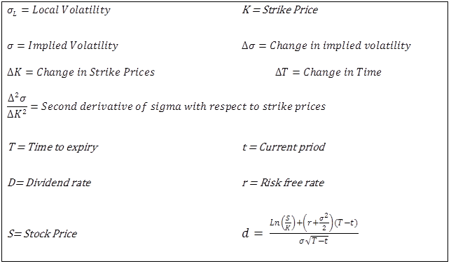
And just in case you were wondering what the fuss is about as well as to get a minor unpleasantness out of the way, here is the discrete form of the equation Schmitz and Rebanato refer to in the above statement.
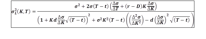
where:
In our next post, we walk through the steps required to produce a volatility surface using the above equation in a market consistent way. Don’t go away, we will be right back (in a relative way) in a few days.
If you would like to learn more, see our latest package on Building Volatility Surfaces in Excel – Study Guide and Excel Spreadsheet template
Credit: Groundwork, research and Excel modeling for this post was completed by Farhan Anwaar, the latest addition to our analytical and content writing team.
xProduct()
Comments are closed.