Building Local Volatility Surfaces in Excel – Lesson Five
So far in our volatility surface tutorial over the last few days we have covered:
- Lesson 1 – Volatility surfaces, implied volatilities, smiles and skews
- Lesson 2 – Volatility surface, deep out of the money options and lottery tickets.
- Lesson 3 – The difference between implied and local volatility – volatility surfaces
- Lesson 4 – Creating the volatility surface dataset using implied volatilities
We now have everything required to build the volatility surface for NVIDIA in Excel.
1) We have the implied volatility data for NVIDIA as of 31 January 2014.
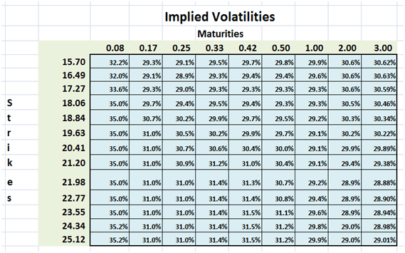
Figure 1 – Implied volatility data from ivolatility.com cleaned up and structured for Surface plot
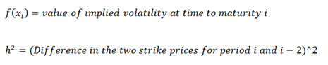
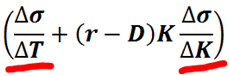
2) We have Dupire’s formula for calculating local volatilities from implied volatilities
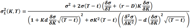
where:
3) Using the continuous form of the Dupire equation we create a discrete variation for usage in our Excel spreadsheet.
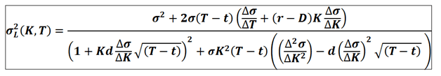
Figure 2 – Dupire Formula – Discrete form
4) In order to calculate sigma’s second order derivative with respect to the strike price K in the equation above, we use a finite difference approximation.
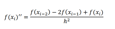
where
5) All that is left now is to follow the process for calculating local volatilities. Four steps remain of the original list. Let go through them one by one.
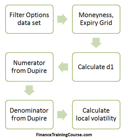
Figure 3 – Volatility Surface in Excel – 6 step process
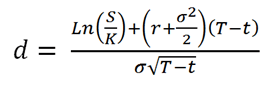
Volatility Surfaces – Step 1 – Calculate d1
We will build multiple grids using the same template used for implied volatilities in earlier lessons. The first grid calculates d1 using the formula shown below. This is the same “d” we use for pricing European options in the Black Scholes Merton Model.
The Excel implementation of the formula is given below.
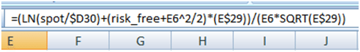
Figure 4 Calculating d1 in Excel
A common spreadsheet error is the incorrect anchoring (using F4) of strike prices (the D Column) or maturities (the 29th row) in the implementation below or missing the anchoring completely.
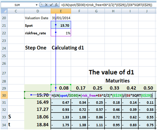
Figure 5 d1 Excel implementation in Strike by Expiry grid
Once that is done, it is a simple copy paste of the original formula across the remaining cells in the grid.
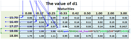
Figure 6 Anchoring the correct cell in the Excel Strike by Maturity grid
The final results looks like the grid below:
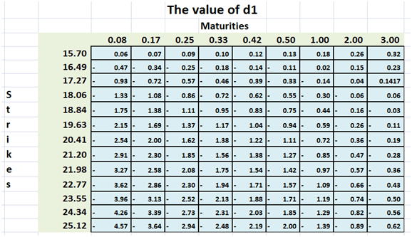
Figure 7 – d1 Excel Grid
Step 2 – Calculating the first and second order rate of change
Using finite difference we now calculate our two first order and one second order rates of change used in Dupire formula. We use the same sequence of steps to create three more grids. One each for each rate of change.
The two first order rate of change are sigma with respect to changing maturities and sigma with respect to changing strikes:
The Excel implementation for both is shown below:
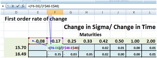
Figure 8 First order rate of change – Sigma by Time
Notice the empty first column. You need two results to calculate the first order difference.
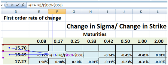
Figure 9 First order rate of change – Sigma by Strike
Here the first row is empty. Once again you need two results to calculate the first order difference hence the empty first row in the grid.
The second order rate of change (sigma with respect to strike) gets used in the denominator and is shown below:
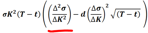
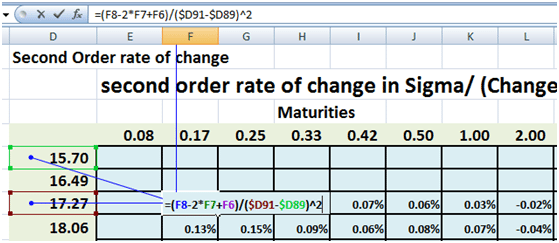
Figure 10 Second order rate of change – Sigma by Strike – Using finite differences
Since you need three values for the second order change, the first two rows will be empty.
The final values of the second order rate of change in the grid are shown below:
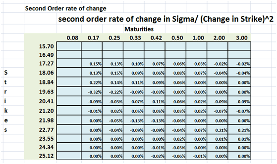
Figure 11 Second order finite differences – final grid
Step 3 – Calculating the numerator and denominator
All that is left now is the to calculate the numerator and denominator in the grid using Dupire’s formula and we are done. We use the same sequence of steps to create three more grids that calculate the numerator, the denominator and the local volatilities and show the Excel implementation as we move forward.
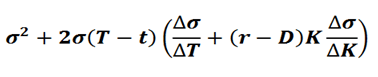
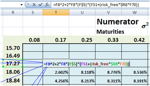
Figure 12 Dupire Formula – Numerator calculation in Excel grid
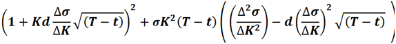
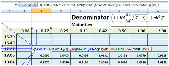
Figure 13 Dupire formula – Denominator calculation in Excel gird
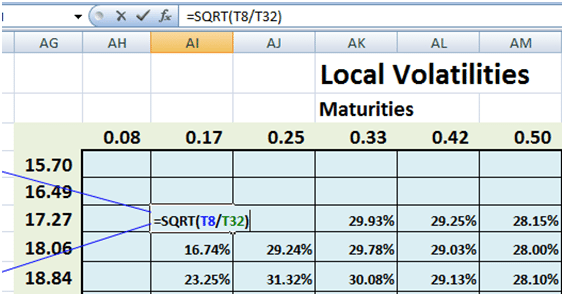
Figure 14 Local volatility calculations in Excel grid
The last and final step leaves us with a grid of local volatilities that vary by Strike prices and Maturities.
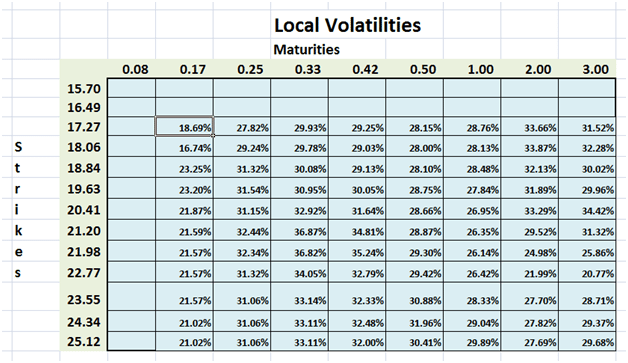
Figure 15 Local volatility surface grid – final results
Step 4 – Plot the surface
Select the local volatility grid that you have just created. In your Excel Tool Bar:
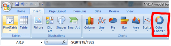
Figure 16 3D Surface charts in Excel – Step 1
1. Click on Insert
2. Pick Other Charts
3. Click on 3D Surface
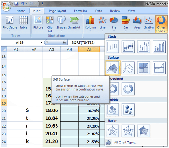
Figure 17 3D Surface charts in Excel – Step 2
That is it. You are done. Your local volatility 3 D surface chart is ready for review and presentation
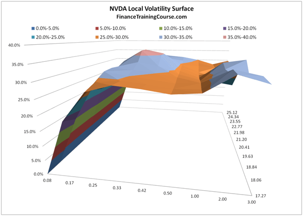
Figure 18 Local volatility surface in Excel – final results
While we can now all take a bow for completing the volatility surface plot in a tool like Excel, the real work has just started. How do your interpret the volatility surface diagram above? How do you go about putting it to work? What about implied forward volatilities? How do they relate to the work we have just done.
Think about these questions while we dream up our next big teaching assignment.
Comments are closed.