Unexpected Loss (UL), Expected Loss & Economic Capital

9 mins read

A follow up post on our Economic Capital series where we looked at an alternate approach for calculating Economic Capital using accounting data rather than the BIS guidelines. Within that discussion, it was felt that we needed a review of BIS guidelines on Unexpected Loss (UL), Expected Loss (EL) and Economic Capital (EC) to make a more appropriate comparison of EC methods and tools.

After all without understanding the process of calculating unexpected loss using the BIS model how could we really appreciate the solutions the alternate approach offers when it comes to Economic Capital modeling.  

1. Economic Capital & Expected and Unexpected Loss

In the banking world, economic capital approaches use a model based on the value at risk.  Within the regulatory framework, economic capital should compensate for unexpected and unanticipated losses booked when banks and financial institutions are forced to function outside their normal operating environment.

To estimate economic capital the model breaks the return distribution down into two segments. A likely, expected loss and an unlikely unexpected loss.  Unexpected loss is estimated by setting an extremely high threshold (unlikely probability).  The difference between unexpected and expected loss serves as an estimate for economic capital.

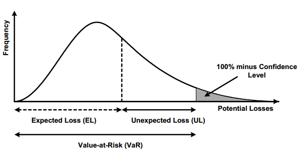
Regulatory guidelines suggest the expected loss figure is determined by the midpoint of the loss distribution[1].  BIS approach assumes that reserves and provisions held on the balance sheet of the bank should adequately cover and compensate for “expected” loss caused by normal operating conditions and economic capital should primarily cover the “unexpected” portion of the loss distribution.

2. Dataset & distribution

For the model to work we need a reasonably sized data set and some stability in the return distribution. For instance, if we plan on using the 99.9% threshold for unexpected loss, a dataset with only 30 data points won’t be effective. The resulting distribution wouldn’t have the granularity we need to answer basic questions focused on how predicted loss numbers would change as we walk up and down the distribution.

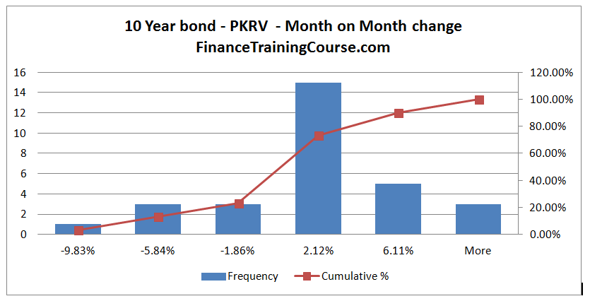
For example, the monthly return distribution of interest rate changes in a 10 year emerging market sovereign bond does not have sufficient details to build a complete economic capital model because the model is missing definition (details) required to calibrate the model at different probability thresholds (99%, 99.9%, 99.99%). At 99% percentile, we need 100 data points for the model to work. For a configuration requiring 99.9% or 99.99% percentile, we need 1,000 and 10,000 data points respectively.

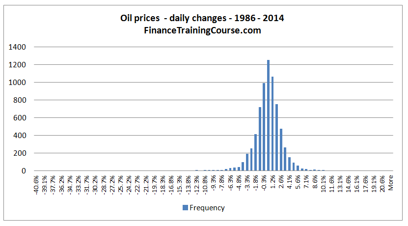
A distribution with twenty eight years of daily price change data for crude oil price has 7250 rows of data and can be configured to model capital at the 99.9% threshold, possibly a bit higher.

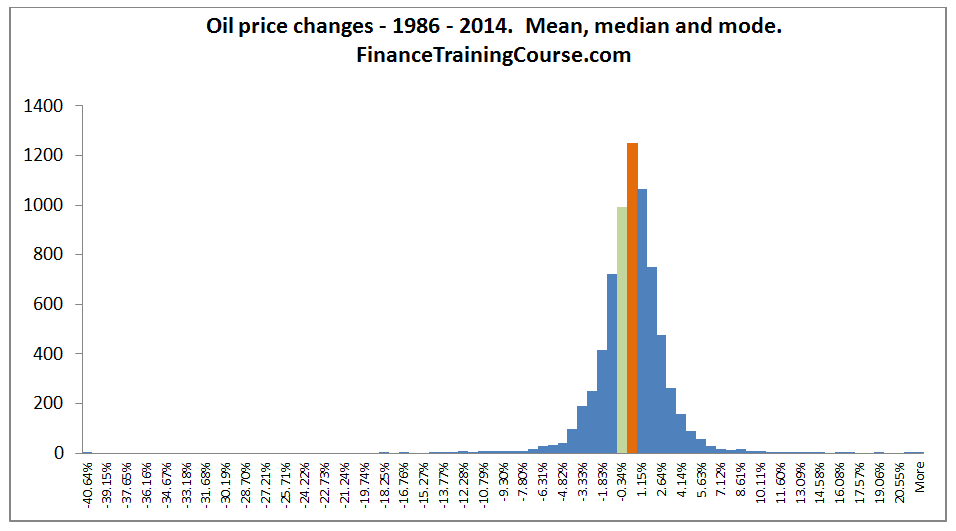
But granularity is not the only consideration. Using the oil price distribution as an example we need to understand how returns are distributed, the shape and form of the distribution and expectations (mean, median & mode of the return distribution).

3. Credit Risk

How do we extend this approach for estimating economic capital for credit risk?

The credit risk methodology uses three estimates. Probability of default (PD), Loss Given Default (LGD) and Exposure at Default (EAD) for a given asset class. Once the estimates are available we also need to factor in the correlation between line items in a given asset class as well as across asset classes.  That is a big issue given the number of product types and subtypes available on the credit side and an equally impressive list available on the investment side. Making them all work together on a UL calculation for an economic capital model is an awkward task.

4. Calculating Unexpected Loss – A simplified case study

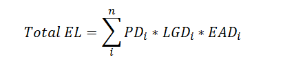
Our starting point for estimating Expected Loss (EL) is the following equation:

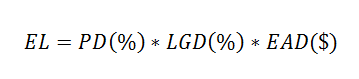
Let us take a look at each of these components individually.

a. Probability of Default (PD)

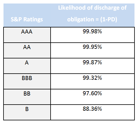
The probability that a default will occur on a credit obligation by a client leading to a partial or total loss.  Probability of default estimation models use a combination of behavioral data (past payment trends and history), financial information (leading indicators based on financial ratios) and subjective information (auditor profile, market feedback) to estimate PDs. Rating agencies use slightly different models to estimate PDs for a given rating class. For instance, the original S&P model bases credit ratings on their internal assessment of default by a given name:

b. Loss Given Default

The conditional expectation of loss given that default has already occurred. The LGD estimates vary depending on the underlying transaction, committed collateral, security and claim type of a loan. LGD could also be expressed as (1 – RR) where RR stands for recovery rate. LGD also becomes important when in addition to rating obligors, we also rate facilities.  Also, see E Altman Default Recovery rates and LGD in Credit Risk Modeling and Practice (2009).

c. Exposure at Default (EAD)

An estimate that measures the exposure of a counterparty at the time of default. Imagine a working capital, overdraft or running finance line originally approved for  1,000,000. At the point that default occurs would this line be fully drawn, partially drawn or completely undrawn? A funded line of credit or commitment is relatively straight forward, but unfunded and contingent exposures are a little more complicated.

A forward contract on a foreign currency comes with local currency exposure that changes with changes in exchange rates. As rates go up and down the replacement cost on the contract if a default occurs also moves. Multi leg interest rate and cross currency swaps are more because we now begin to deal with multiple benchmark rates at multiple points in the future.  For such exposure a simple replacement cost estimate at a given point in time is not sufficient, we need to evaluate the worst case exposure across the life of the transaction (aka potential future exposure).  See EAD calibration for corporate credit lines – 2009.

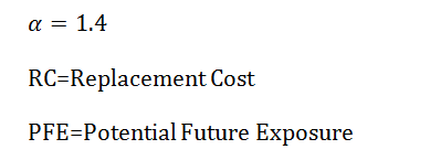
When we put all of these considerations together, the Exposure at Default (EAD) value is modeled as under:

For normal conventional lending products:

EAD = Drawn portion of the line  + Loan Equivalent Amount (LEQ) * Undrawn amount

For derivative, unfunded and contingent exposure:

Where:

5. Expected Loss, Unexpected Loss for derivative exposure

In our sample unexpected loss case study we will use publicly available financial statement data for a large bulge bracket investment bank and try and estimate expected loss (EL), unexpected loss (UL) and capital requirements using the approaches discussed above. We will make a number of simplifying assumptions and use shortcuts to improve readability.

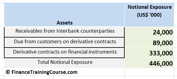
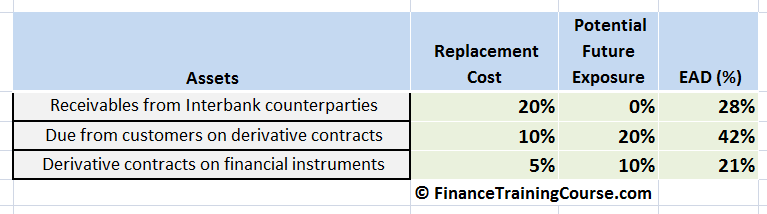
We start with notional exposure (expressed in ‘000 US$) to derivative contract counterparties under the following categories.

a. EAD and EL calculations

Using the above exposures and the preceding model for estimating EAD (exposure at default) for derivative contracts we end up with the following values for EAD.

Using our EAD estimate from above we also add the probability of default (PD), loss given default (LGD) and notional exposure in dollar terms to estimate the expected loss figures for each of the above mentioned line items.

The Expected Loss (EL) amount is calculated using the Expected loss equation

b. Calculating Unexpected Loss (UL) using the short form approach

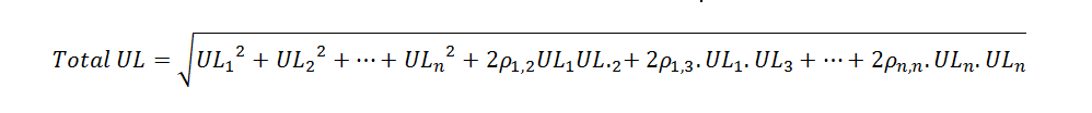
The equation for the calculation of UL needs some work.  See Measuring economic capital using loss distributions[1] paper on the more detailed mathematical derivation. For a single credit exposure, Unexpected Loss (UL) is  given by:

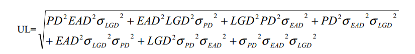
Where:

PD = probability of default

EAD = Exposure at time of default

LGD = Loss Given Default

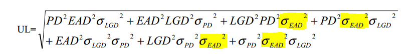
Within the above equation, EAD is deterministic (known) and hence has a variance of zero. That reduces the equation from seven terms to three.

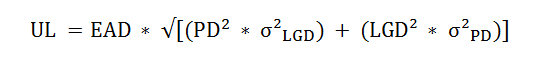
We take EAD out of the square root, ignore the smaller terms and are left with:

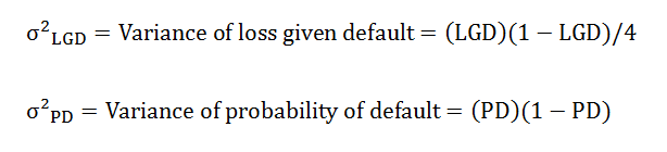
Where PD is assumed to follow a Bernoulli distribution and LGD follows a beta distribution and hence leads to:

Where:

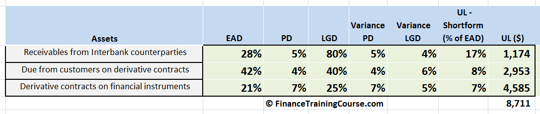
Putting all of the above to work together gives us our first estimate on Unexpected Loss (UL) using the short form approach.

c. Calculating Unexpected Loss using the BIS method

The BIS Basel standard method for capital charge calculation is a little different. Ignoring the impact of correlation the BIS approach essentially calculates unexpected loss at 99.9% threshold, subtracts the expected loss given by multiplying PD x LGD x EAD and uses the difference as its estimate for the capital requirement.  There are a number of adjustments made in the formula for maturity and correlations but we will ignore these for the purpose of simplifying presentation in our case study.

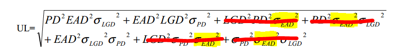
The full form of the capital charge equation follows. Please see An explanatory note on the Basel IRB Risk weight function for a more detailed treatment.

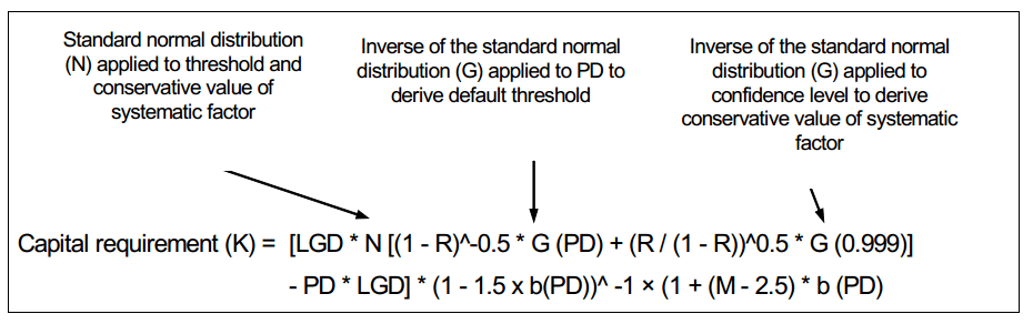
Color coding the above diagram shows the relevant sections of the equation

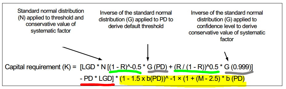
1. The section of the equation underlined in green deal with the correlation adjustment within the asset class
2. The grey underlined components calculated the EL and UL at 99.9%
3. The yellow highlighted section is the maturity adjustment
4. The red underlined section is the EL adjustment from the UL result

Model implementation in EXCEL

Assuming zero correlation and plugging in our EAD, LGD and PD values in the above equation we get the following model implementation in Excel.

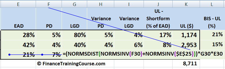
We take the z-score for our current estimate of PD, add the 99.9% z-score to it, add both numbers to calculate the revised worst case PD and multiply the result with EAD and LGD estimates for that line item.

Zooming out and repeating it across the three exposures we have been following in this case study we get:

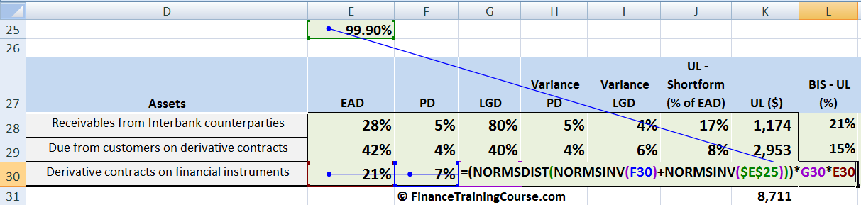
BIS UL in column (6) is the BIS estimate for unexpected loss. Economic Capital (B) in column (7) is the adjusted capital charge after deducting the expected loss calculated in column (2).

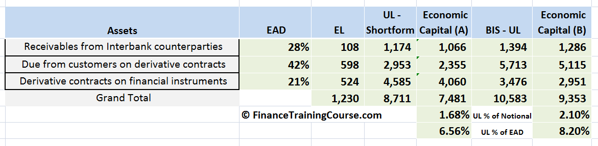
The short form approach understates unexpected loss (UL) for the dataset used in the case study. The BIS approach leads to higher UL as well as higher capital charge estimates in our simplified model. Plugging in correlation estimates should help bring the numbers closer together because we do use them in the short form approach but ignore them in our contrived BIS example.

Remember our original disclosure. This is a simplified presentation assuming zero correlation and using a model for single credit exposure.  When you extend UL for multiple exposures or across multiple asset classes the equation becomes quite intimidating and daunting.

Footnotes

[1] Osei Antwi, Alice Constance Mensah, Martin Owusu Amoamah, Dadzie Joseph. Measuring Economic Capital Using Loss Distributions. International Journal of Economics, Finance and Management Sciences. Vol. 1, No. 6, 2013, pp. 406-412, January 2014.

[2] With statistics the mean of a distribution represents the average (expectation), median is the midpoint of the distribution and mode is the most frequent, the most common occurrence. For a normal distribution, all three points coincide at a single point but most real life distributions are skewed and have a different mean, median and mode values. With the Expected loss framework, the expected loss is equated to the median of the distribution.

References

1. “Basel II and the top 5 pitfalls in economic capital modeling”, Sungard: Ambit risk management & compliance, World Finance, 2008.
2. Abolo, Emmanuel, “Basel II and Economic Capital”, Access Bank Plc, 16 Dec. 2008
3. Ashish Dev, “Economic capital: A practitioner guide”, Risk Books, Incisive media investments limited, 2004.
4. Bessis, Joël. Risk Management in Banking. New York: Wiley, 2002.
5. Birge, John R. and Linetsky, Vadim, “Handbooks in Operations Research and Management Science: FinanciaL Engineering”, 1^st, P. 681-726, 2008.
6. Bowers, Newton L., Hans U. Gerber, James C. Hickman, Donald A. Jones, and Cecil J. Nesbitt. Actuarial Mathematics. Schaumburg, IL: Society of Actuaries, 1997.
7. Buck, Eugen and Chorafas, Dimitris N., “Economic capital allocation with Basel II : Cost, benefit and implementation process”, Elseeiver Finance, 2005.
8. Caouette, John B., Edward I. Altman, and Paul Narayanan. Managing Credit Risk: The Great Challenge of Global Financial market. New York: Wiley, 2011.
9. Crouhy, Michel, Dan Galai, and Robert Mark. The Essentials of Risk Management. New York: McGraw-Hill, 2006.
10. Deventer, Donald R. Van, and Kenji Imai. Credit Risk Models and the Basel Accords. Singapore: John Wiley & Sons (Asia), 2003.
11. Dowd, Kevin. Beyond Value at Risk: The New Science of Risk Management. Chichester: John Wiley & Sons, 2003.
12. Farid, Jawwad, “Models at work”, Palgrave Macmillan, Dec 2013.
13. Gallati, Reto R. Risk Management and Capital Adequacy. New York: McGraw-Hill, 2003.
14. Greenbaum, Stuart I. and Thakor, Anjan V. “Contemporary Financial Intermediation”, April 2007
15. Hardy, Mary R., “An introduction to risk measures for actuarial applications”, Construction and evaluation of actuarial models study note, Society of Actuaries, 2006.
16. Hull, John. Risk Management and Financial Institutions. Boston: Pearson Prentice Hall, 2010.
17. Jorion, Philippe, “Financial Risk Manager Handbook”, May 2009
18. Klaassen, Pieter and Van Eeghen Idzard, “Economic Capital: How it worksand What every Manager should know”, 2009
19. Matten, Chris. Managing Bank Capital: Capital Allocation and Performance Measurement. Chichester: Wiley, 1996.
20. Mishkin, Frederic S., “Prudential Supervision: What Works and What Doesn’t”, P. 197-232, National Bureau of Economic Research, January 2001
21. Mulcahy, Rita. Risk Management: Tricks of the Trade® for Project Managers: A Course in a Book. Minneapolis, MN: RMC Pub., 2003.
22. Ong, Michael K. Risk Management: A Modern Perspective. Burlington, MA: Academic/Elsevier, 2006.
23. Painter, Robert A. and Isaac, Dan, “A Multi-Stakeholder Approach to Capital Adequacy”, Conning Research & Consulting.
24. Pearson, Neil D. Risk Budgeting: Portfolio Problem Solving with Value-at-risk. New York: J. Wiley, 2002.
25. Peng, Jin, “Value at Risk and Tail Value at Risk in Uncertain Environment”, Institute of Uncertain Systems, Huanggang Normal University. http://www.orsc.edu.cn/online/090530.pdf
26. Saša Žiković, “Friends and Foes: A Story of Value at Risk and Expected Tail Loss”, Young Economist Seminar, June 2008.
27. Schuermann, Til, “What Do We Know About Loss Given Default?”, Financial Institutions Center, Wharton University of Pennsylvania, April 2001.
28. Sweeting, Paul. Financial Enterprise Risk Management. Cambridge: Cambridge UP, 2011.
29. Van Laere, Elisabeth and Baesens, Bart, “Regulatory and economic capital: theory and practice, evidence from the field”, International Risk Management Conference, May 2009.
30. “Definition of capital”, The Association for Financial Markets in Europe.
31. Navarrete, Enrique, Practical Calculation of Expected and Unexpected Losses in Operational Risk by Simulation Methods, Scalar Consulting, 2006,
32. Proper Risk Assessment and Management: The Key to Successful Banking,Oracle White Paper, October 2012.
33. Holton, Glyn A. “Default Model – Risk Encyclopedia.” Risk Encyclopedia. Web. 22 Sept. 2014.