Copulas – A quick introduction
If you build economic capital models for financial institutions, a common problem is creating a model for the Enterprise. At the simplest level this requires an ability to integrate risk profiles from market, credit and operational risk models. Three different risk categories, multiple risk models, hundreds of assumptions and an integration problem akin to creating a single ring to bind them, to rule them all.
While market risk models come with detail price and return series, credit and operational risk models are not so fortunate. For instances within credit risk, asset valuations may occur on a quarterly or annual basis and we may have significant gaps within the data set. We also need to determine how to model relationship or dependence between retail unsecured credit products (credits cards), retail secured products (housing and auto loans) and corporate credit solutions (term, revolving and project finance loans). Similar challenges exist within operational risk; operational risk types range from items with significant data (treasury limit breaches and ATM downtimes) to items with limited data (loss of business on account of branch unavailability, ) or data capture mechanisms.
While simpler models with Basel II and Basel III frameworks rely on assumptions to reduce the complexity of models, advance approaches as well as Economic Capital models use an advance modeling technique to bind multiple risk distributions into an enterprise risk distribution. The approach essentially takes two distributions and maps the two into a joint distribution. This joint distribution allows you to model the combined risk profile. This modeling/transforming/mapping process goes by the name of copulas. They are used extensively within risk modeling for modeling correlations and dependence and creating joint distributions.
For instance if you were modeling two difference types of operational risks (internal fraud and physical damage to bank assets) and wished to create a joint distribution that would represent the combined operational risk losses from both risk types, a copula could help you create such a distribution. The joint distribution could solve a range of problems for you. To begin with you could a discrete data set and transform it into a continuous form addressing any data gap issues. You could try a range of assumptions around the correlation between the two risk types. You could use the combined risk distribution and use it to create a third joint distribution with another set of risk type distributions from operational, credit or market risk types.
Though fairly simple to implement in Excel once you have the relevant datasets and tools, the language and coverage around Copula usage is shrouded in mystery. Like most continuous models the application papers use a fair bit of mathematical transformations. Compared to option pricing there is no PDE mathematics but if you are allergic to equations, there is a reasonable chance that you would look the other way or simply switch to a different path when forced to cross roads with the subject. In our series of building and using copulas within risk management we create a simplified step by step walk through including introductory and fairly detailed example that shows how to build Copulas in Excel. While the example we use rely on commodity prices (WTI and Brent, Gold and Silver), the approach can easily be extended to non-market risk data series.
If you are interested in a more detailed treatment, please take a look at the attached bibliography at the end of this paper that includes some of the more useful and interesting efforts in this field. Our hope is that our simplified example, terminology review and bibliography reference will turn out to be a useful resource for individuals interested in learning more about the subject without requiring advance graduate studies in statistics, applied calculus or computational finance. If you have any feedback or comments on improvements that can further simplify the treatment and our presentation, please feel free to share it with us.
Building Copulas – Statistical Terminology reference
We begin with a short review of statistical terms that we will be used frequently in our Copula tutorials. Advance users can skip this review.
Statistical Distributions
A distribution models or gives us an indication of what to expect with respect to a certain phenomenon or variable. For instance we were to build a model of daily oil prices (WTI – West Texas Intermediate Crude Oil) changes over the last few years we could use historical price changes to build such a model.
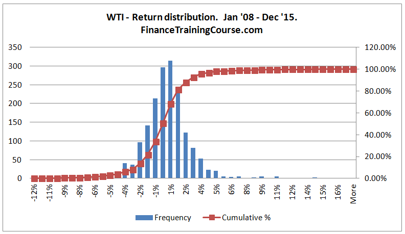
The above histogram shows that that range within which daily oil prices are likely to move as well as the most common price changes we should expect. A histogram is one representation of a distribution. A distribution may also be written down in a discrete form in the shape of rules or continuous form in the shape of a mathematical equation. Such a model would assign a variable (X or Y) to daily oil price changes and then write out the relevant rules that can be used to model its behavior. If we wished to simulate all price changes we could use the actual distribution represented by our histogram, or use the discrete or continuous form.
Uniform distribution
Our oil price changes distribution showed us that some prices changes are more likely than others. For instance if we take a second look at the same image we can say that oil prices are more likely to move within a +2% -2% range on a daily basis than a more extreme move. Alternatively the probability of oil prices changing by 1% is significantly higher than it changing by +10% or -10%.
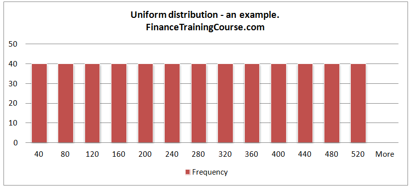
A uniform distribution is a distribution where all events/points are equally likely to occur.
Marginal and Joint Distributions
Our histogram above for daily oil price changes using WTI as a benchmark models a single variable – WTI. If we wanted to model Brent, we would need another distribution and the results would look a little different. If we assigned a variable X to model WTI, we would now need a different variable Y to model Brent.
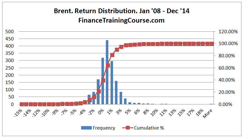
Even though the two distributions look similar when you look closely you will see that there are differences in how the two distributions are centered as well as in terms of their extreme values or tails (maximum positive and minimum negative changes).
The distribution of Brent as well as WTI when looked and evaluated in isolation will commonly be referred to as the marginal distribution. If we were modeling a portfolio of two positions in WTI and Brent, we would need to model or build a joint distribution. A joint distribution would require us to factor in a weight for each position as well as include a joint model.
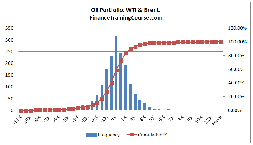
We can see that the joint distribution of WTI and Brent is a little different from the individual marginal distributions. With the world of Copula are focus is using marginal distributions to build joint distributions using what some would call a simple transformation exercise.
Correlations and Regression
If we wanted to use the price of WTI to predict and forecast the price of Brent we would need to dig a little deeper than just the distribution. We would need to better understand the relationship between WTI and Brent. Ideally if we gave our predictive model the current price of WTI, the model should forecast the new price for Brent. This relationship or dependence between the two data points needs to be modeled.
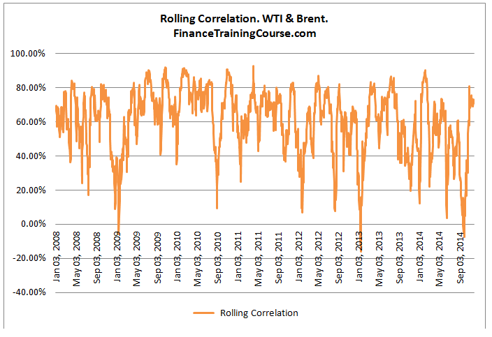
Based on our original data set we would expect that the two data series would be strongly correlated. But that assumption is based on how we calculate correlations. If we just measured correlation over the entire six year period of observations we could a number between 55% – 60%. If we modeled correlations on a rolling 30 day basis we would get the series that we see below.
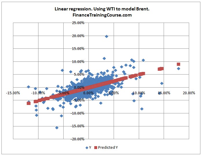
Alternatively if we used the Excel regression function to plot a relationship between the two series using the entire 6 years of data, we would end up with the image below which suggests that for the data set in question there is a strong linear relationship as far as the regression model is concerned between WTI and Brent. Such a linear relationship is also known as linear or Pearson correlation. To correctly measure a non-linear relationship we would need to use Spearman correlation.
This concludes our first lesson and review. In our next lesson we will start work on specifying the theoretical foundations for building Copulas in Excel. Also see Aggregating risks for ICAAP – Copulas at work and Using Copulas in Excel to model the spread between WTI and Brent.
If you are exploring the use of Copula for modeling Bank Capital or managing the correlation between different risk types (Market, Credit, Liquidity, Operational Risk), take a look at our Economic Capital series that uses a Copula free approach to estimate Economic Capital for internal reporting including ICAAP.
Understanding Copulas. A short bibliography
- Defining Copula. John C. Hull, Risk, October 2006.
- A brief introduction to Copulas.
- Copula and credit models.
- Understanding relationships using Copulas.
- Copula for Finance. A reading guide and some applications.
- Copula concepts in Financial markets.
- Copula Theory. An application to risk modeling.
- Modeling Copulas.