We dry run of our Portfolio Optimization model for different allocation strategies and evaluate their performance post allocation. We introduce and use the concept of holding period return over two different observation periods. Four different portfolio allocation strategies are considered, labeled strategy A, strategy B, strategy C and strategy D.
How to calculation holding period returns?
To evaluate the results and compare the four strategies we calculate holding period returns for the securities in our universe. We would like to measure the holding period return across two observation periods. The first is the historical period of our dataset which we use for portfolio construction; in our case is 8 years ending on 30th June 2016. The second is our performance horizon; from the point of allocation 1st July 2016 to the point of review which is 31st October 2016.
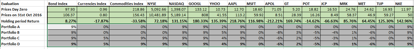
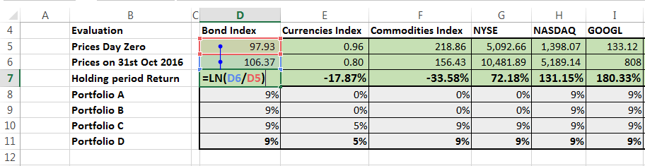
To calculate the holding period return over a period, pick two dates – a start date and end date. Pick closing rates for both dates for all the securities in the securities universe. Then apply the return formula Natural Log or ln(End date price / Start date price) for all securities. The resulting series gives you the holding period return over the observation period.
For equities security prices can generally assumed to be dividend adjusted. But you should double check with your data source if this is the case. For bonds and currencies, we can add coupons and deposit rates as a source of additional income over the holding period. For commodities, if we are trading nondeliverable or cash settled future contracts, there is no cost of carry. If we are trading and holding physical commodities a cost of carry has to be deducted.
Portfolio construction versus portfolio evaluation
There are two key points that we would like to make. When we allocate portfolios and compare results of one strategy with another, our portfolio metrics figure is calculated looking back in time. For instance when we compare the results of Strategy A with B and C, we see a big difference between A and B, but not that great a difference between B and C. We want to emphasize that this assessment is based on historical performance and there is no guarantee that we will see the same performance figures in the future.
It is only when we let the portfolio run with market conditions does the robustness of our allocation comes to fore. Till then our best case assumption is that the future will be just like the past. If that assumption holds our portfolio will do well, but if it doesn’t our performance will be disappointing.
For portfolio construction purposes, we have only used the data till 30th June 2016 for a specific reason. We want our allocation to be independent of the most recent four months of market performance. The idea is to use market performance in the July – October period as a forward looking evaluation dataset for our different strategies.
While Strategy B and Strategy C may seem very close when we look at the historical data set, it is their performance in the forward looking data set that we want to use as a scoring and grading mechanism.
For the purpose of our initial analysis, we will ignore bond coupons and dividends but we will come back and revisit the topic of incorporating dividends and coupons in our return calculations in a later note.
Portfolio allocation strategies
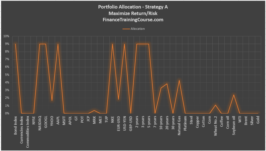
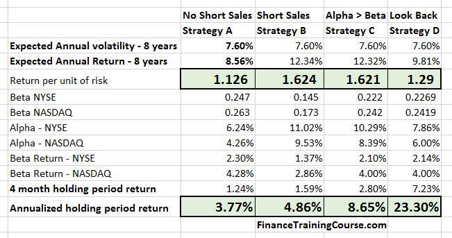
- Assumes there are no short sales and maximizes return per unit of risk. – Strategy A
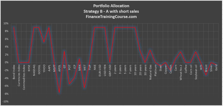
- Assumes that short sales are allowed and maximizes return per unit of risk. – Strategy B
- Maximizes return per unit of risk with short sales and with portfolio alpha > portfolio beta – Strategy C
- A look back C. For the 4-month period, 1st July to 31st October 2016, pick securities that maximize holding period return – Strategy D
Our solver model for Strategy C and D forces Alpha excess return to be significantly higher than Beta and at the same time requires a minimum projected Beta return of 4%.
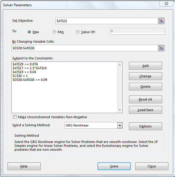
All four options limit allocation in a single position to less than 9%. There is also a limit assigned to maximum volatility – 9% but the actual optimal portfolio volatility can be lower.
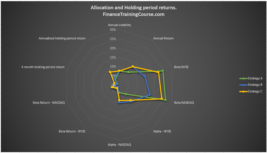
Holding period returns during the allocation/ construction period
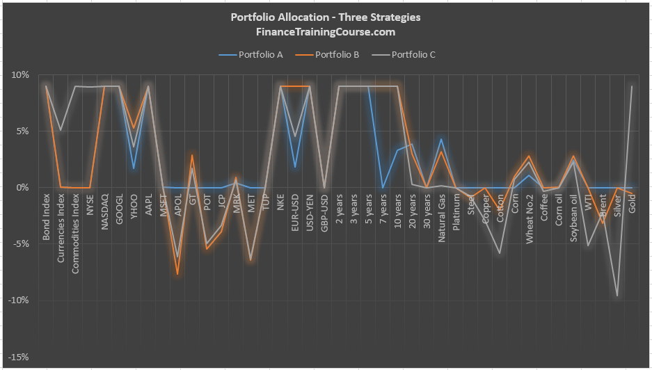
When we run Solver with the three options here is what allocation and initial results look like at the point of allocation
Strategy A
Strategy B
Strategy C
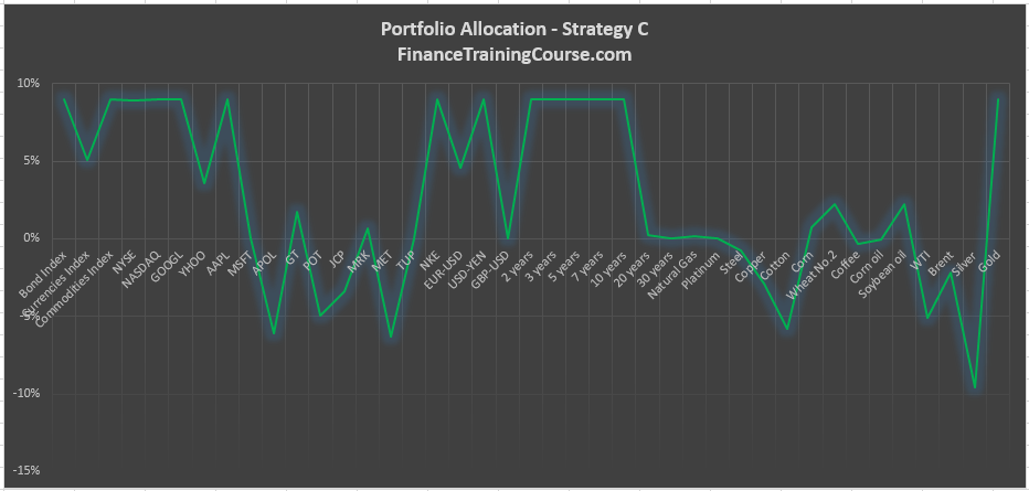
B and C are quite similar except for our little hack with Alpha.
Now let’s run the three on the forward looking July – October data set
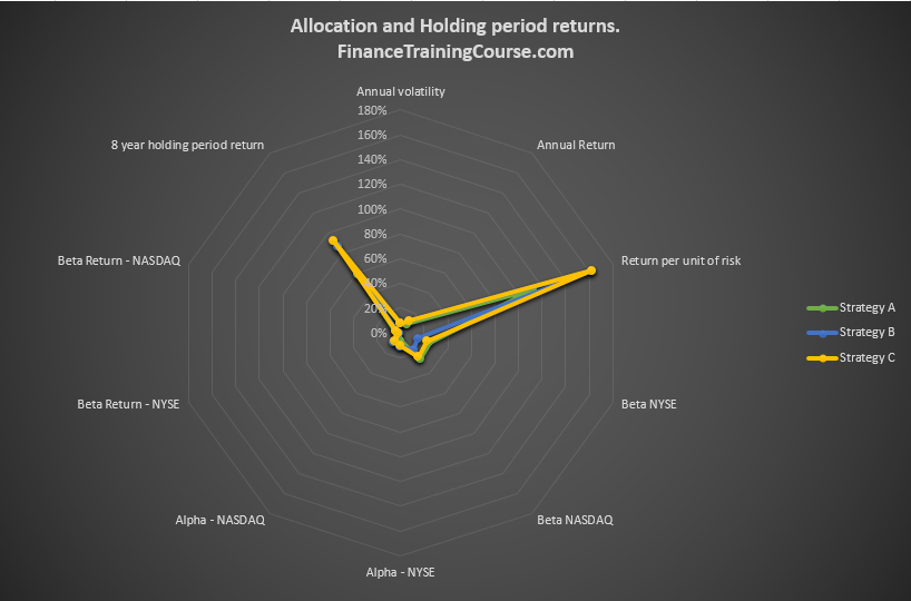
You can clearly see the difference if you look at the holding period return over the 8 year period.
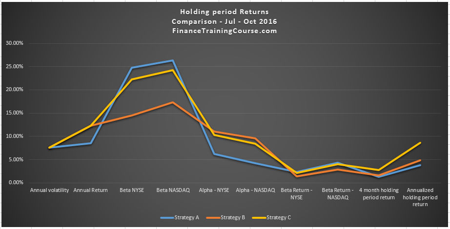
Holding period returns during the evaluation period
That difference becomes even more clear when we switch to evaluating holding period return over our 4 month observation period.
C has clearly out performed B. This, despite the fact that the original portfolio metrics limited to risk and return didn’t lead to significant differentiation between B and C (other than the Alpha hack), over the 4 month period. And the numbers are more impressive when we annualize them.
However, before we congratulate ourselves, note that the annualized return for both strategies is significantly lower than the expected average annual return calculated using the 8 year dataset. Do we know why that is? Do we?
Holding period returns for the revised construction period
If we restrict our allocation data set to the last two years, the suggested allocation by Solver will change dramatically. Using an 8 year allocation window, average out performances for both Apple computers and Yahoo and doesn’t completely highlight the impact of the recent downtrend in their prices. It’s not just Apple and Yahoo, within commodities markets also there has been a price route of sorts beginning November 2014. Currencies have also been in turmoil. Both the Yen and the Euro are heading in very different directions post the events of Brexit. In the US, there are rate hike expectations in the Treasury markets for the last two years.
Restricting the horizon to just the last two years allows us to allocate a significantly better portfolio.
Strategy D – Allocation based on a forward looking data set
We can actually do better by taking our model one step further. Rather than allocating using our eight year backward looking set, we can allocate using our forward looking data set to find out the best of all possible allocations, given the recent four month performance of securities in our security universe. We will call this allocation Portfolio D. Our portfolio allocation with the benefit of look back over the last 4 months.
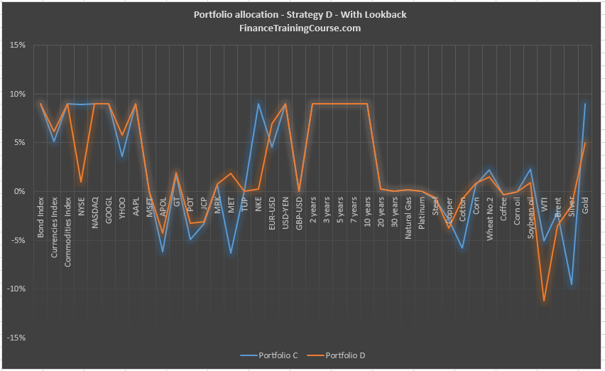
When compared with Strategy C, D tracks it except for a few key differences. The shorts are deeper when it comes to oil and the long position is more substantial in Gold.
What generated this performance? What was the contribution of each component of the strategy to the total portfolio return? This is a key question that we must answer when we dissect the performance of each one of our strategies. We take a look at strategy D below. Repeat the analysis for the other three portfolio strategies as a homework assignment.

From the EMBA Portfolio Management and Optimization course run at SP Jain’s Dubai campus. Also, see the Portfolio management course resource page.