There are a number of changes that we need to make to our existing model before we can build the solution for life insurance portfolio optimization challenge. As mentioned earlier, the insurance portfolio challenge comes with additional requirements that emphasize the structure of our liability portfolio much more than the return. Our objective is to seek an investment allocation that will protect our existing surplus, rather than maximize holding period return. If you remember surplus in the life insurance investment fund case was defined as the difference between asset and liabilities and we wanted to minimize changes in the surplus on account of interest rate movements and asset liability mismatch.
This is the crucial difference between the work we have done so far and this challenge. This is the first time that we are looking at both sides of the balance sheet – assets as well as liabilities. While for illustrative purposes we have simplified the presentation, the principle of matching duration of assets with liabilities remains the same.
The changes in our model include:
1. Adding bond duration, convexity, yields and liquidity data for Treasury bond securities in our portfolio.
We first need to calculate and tabulate duration and convexity estimates for each of the bonds in our universe.
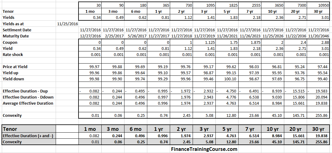
Then link the tabulated values to the model.
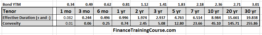
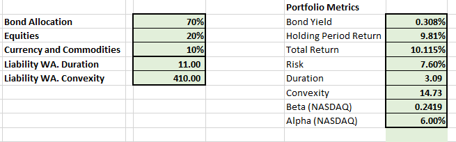
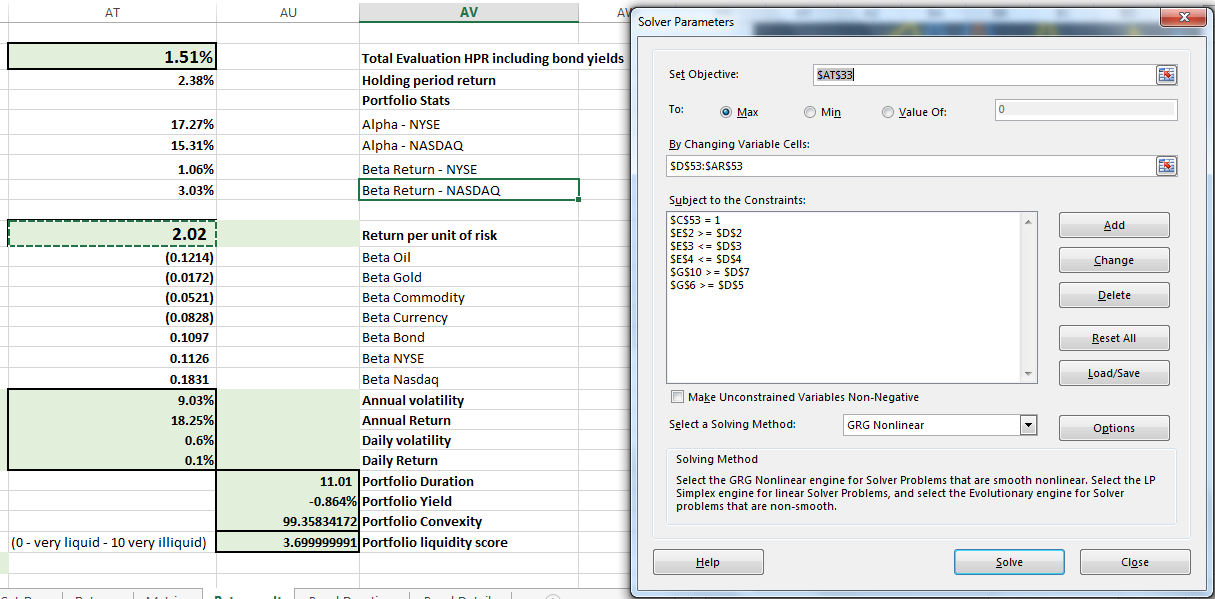
We add the duration, convexity, yield to maturity values just above the allocation row in our model. We add the liquidity data in the row just above portfolio allocation. For liquidity we are using a simple grading scale that goes from 0 to 10. 0 is our most liquid asset and would represent bills and liquid currency positions. 10 is our least liquid position and may include long term bonds and small cap equities or equities or securities that are under a cloud and therefore have limited buyers interested in picking up large quantities.
2. For each of the above metric, we need to calculate the applicable results for our portfolio.
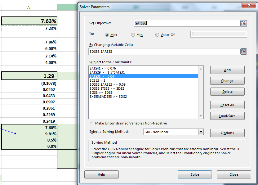
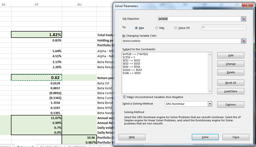
3. We also need to set up a constraint calculator that can make it possible for Solver to apply the required constraints on portfolio allocations.
For this, we need a calculated cell that sums up total bond, equities, currency and commodity allocations.
4. Update the solver model to take into consideration the additional constraints specified by our investment policy document and remove constraints specified by earlier solver models.
A common mistake is to simply limit all allocations by some value. That doesn’t work well. Solver won’t be able to work with the above model because some of the constraints are not defined correctly.
The model, on the other hand, gives us the desired result and is cleaner to implement as well as explain.
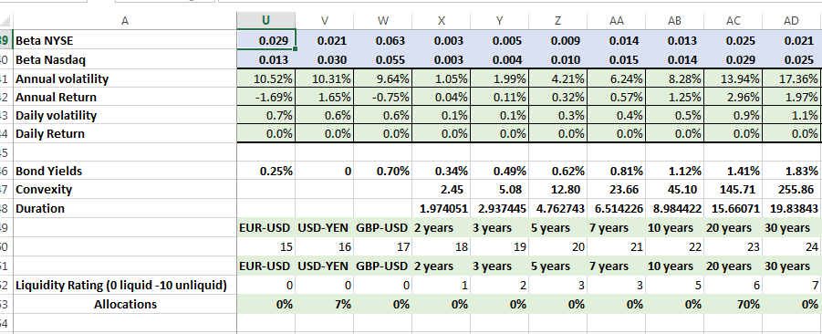
Once the changes are made running the solver model to create an optimized portfolio recommendation doesn’t take long. Remember that unlike prior portfolio management exercise – this time the objective is not excess return or optimal return but limiting changes in the portfolio surplus because of changes in the interest rate environment. It will lead to lower returns but a better asset liability match. We use the duration and convexity constraints to achieve this goal.
We evaluate three separate solutions
- One – allocations with short sales allowed – this allows for the best returns but may not be a valid solution given the conservative state of insurance company investment policy requirements.
- Two – without short sales – more likely and real but lower returns
- Three – maximizing holding period return from an evaluation holding period return point of view
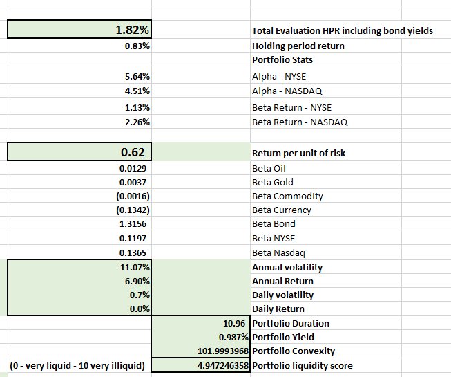
Our initial solution leaves a lot to be desired compared to some of the earlier portfolios we have seen in this course but that is the nature of the life insurance business. One could make a point that even from a volatility or return per unit of risk basis also the portfolio results are underwhelming. Also note that while we have come close to matching duration, we are still short and that we have failed completely on the convexity matching side. One big reason for this are embedded options within life insurance liabilities that make it difficult to hedge convexity by conventional products. If we are serious about matching convexity we may need to explore the interest rate options world to offset the convexity gap between assets and liabilities.
The question is if this is the baseline result, are there any formulations where you could generate a better performance?
If we add the option to explore short sales, the numbers change dramatically but convincing a conservative board to work with short sales is going to be a different challenge.
Consider that your next assignment. Given the constraints of the model specified in the challenge as the results shared here, create a solver model/constraint combination that holds true to the mandate and yet improves on the results suggested and shared above.