A guide for adding Monte Carlo simulation to financial models in EXCEL to enhance stress testing and scenario analysis.
Remember our friendly e-commerce store that shared its live data for our growth in a pandemic series? How or why should we add Monte Carlo simulation to our growth analysis financial model?
Simulation does the same thing generating the distribution did for us. It makes it possible for us to come with a broader range of values for stress testing and scenario analysis. Our ability to do that is limited by our imagination and world view. Simulations broaden it up.
If you are a brand new venture with no prior data, numbers or figures but have industry benchmark and metrics, simulation is a good starting point. When used correctly it can give you a range to work with for your model.
In this specific case, we are standing at Feb 2020 wondering what the rest of 2020 is going to look like. Our historical data set and models have been rendered irrelevant because no one knows what March is going to look like. We need a new model.
For our e-commerce startup, we will use simulation to answer the same question. Standing in Feb 2020, should we expect growth or decline in orders for the full year 2020? Here is our historical dataset.
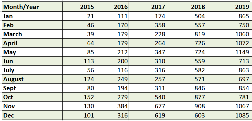
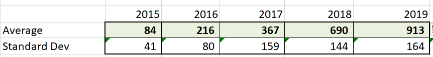
Step One – Calculating Means and Standard Deviations
Calculate averages and Standard deviation by year. We do that by using Excel functions for both metrics. This give us baseline numbers to calibrate our model with.
Step two – The Sales Funnel
Our alternate sales model is traffic based. It follows the standard funnel approach from impressions to revenues. Impressions > Click through rate > Clicks > Conversions > Orders > Ticket Size > Revenues. We will simulate part of the funnel to model revenues.

Historically our e-commerce site scores 9 million to 12 million search impressions a year. A click through rate that ranges between 4% and 8% and landing page conversion rates of 1% to 1.5% Order sizes range from 500 to 5,000 For our first pass we assume a simple model.
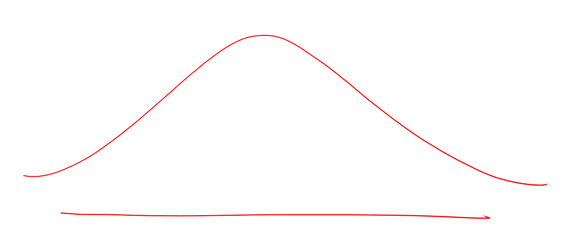
We will simulate click through rates, conversion rates and ticket size to get to simulated revenues for 2020. Our first model will assume all three variables are normally distributed. We can revisit and change this assumption later.
Step Three – Setting up the Monte Carlo simulation model
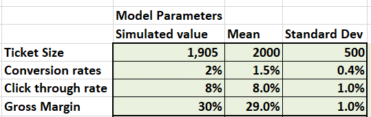
We need to setup a simple simulator that can give us simulated values for our model parameters. Which we can then use to predict and forecast model revenues. We plug in a sample set to check if resulting values tie in with expectations.
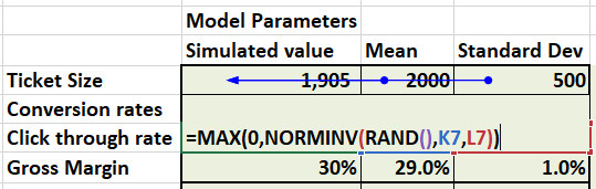
Step Four – The formula
We use Excel NORMINV function to simulate sampling from normal distribution. The RAND() function gives us a random number between 0 and 2 which NORMINV() function converts to a normally distributed random variable using mean and standard deviation.
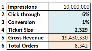
Step Five – Plug in results
Plug in simulated results into the funnel. 10 M impressions * simulated click through *simulated conversions * simulated order size = Revenue for the year. Plug this in your financials and you have simulate revenues.
Step Six – Store the results of the Monte Carlo simulation
The only challenge left now is how to store the simulation results. Each simulation run is a single value that by itself is not worth a lot. It is an iteration. It is only when you can store and compare multiple iterations that you can find meaning from the run above.
Each time we press Enter or F9, Excel generates a new set of random numbers and updates the table above. That number represents a single trial. We need a collection of trials to get a meaningful answer.
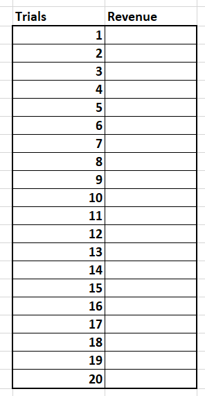
Meet our data store.
A simple table with number of trials on the left and results of the trial stored on the right. Ideally we want Excel to fill this in on an automated basis. We may also want to store a few other metrics for each trial from our simulation model.
Depending on how volatile your distribution is and how complex your relationships are, we can get by with 500 to 5000 trials.
Stability in results from a benchmarking perspective is achieved when a certain condition is met. We will discuss the condition towards the end of our discussion.
For our answer we average out the trials. Build a table as shown below and link the header cells to your simulator.
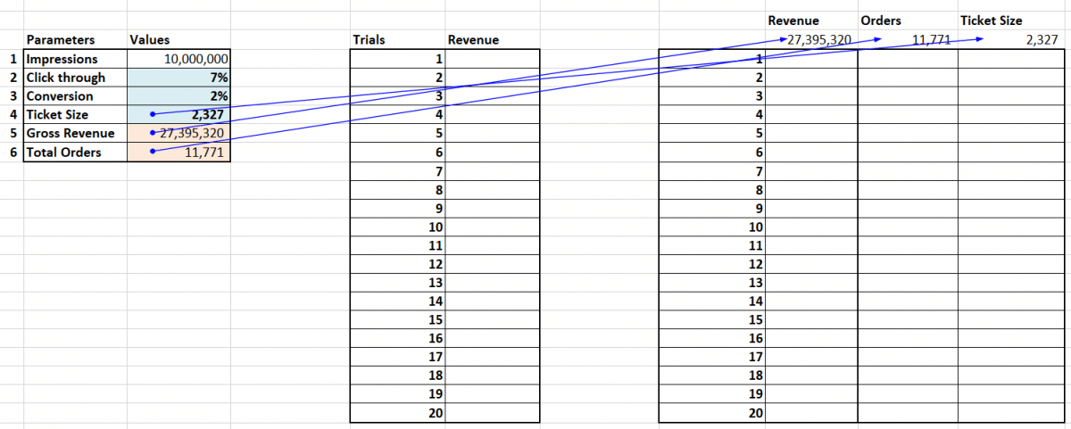
Then under Data, pick What if Analysis and Data Tables. If you don’t have the tab go to File>Options>Add-ins to activate the data analysis tool pack.
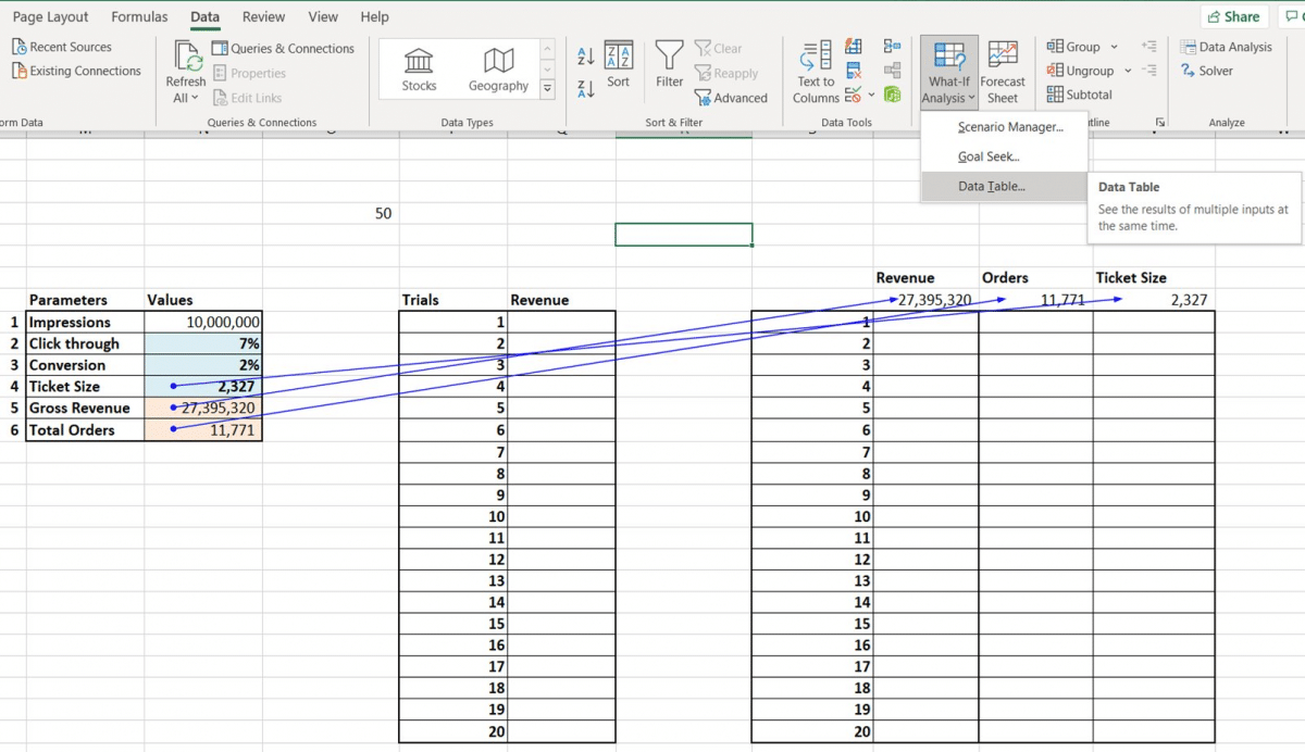
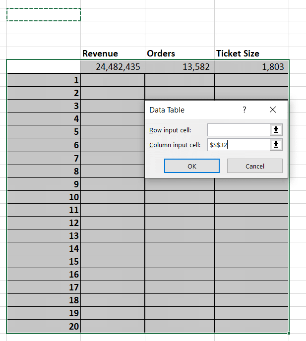
Select the table as shown below and under column input cell pick a blank Excel cell. Press enter and Voila! Congratulations you have just made Excel generate and store 20 iterations automatically for your simulation model.
Step Seven – Build a profile
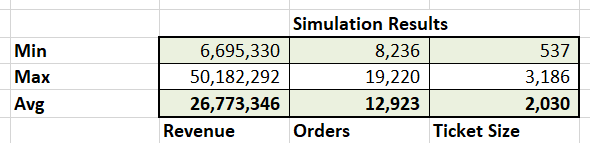
For your final step Calculate average, minimum and maximum values from the 20 trials you have just run to build a profile for your business.
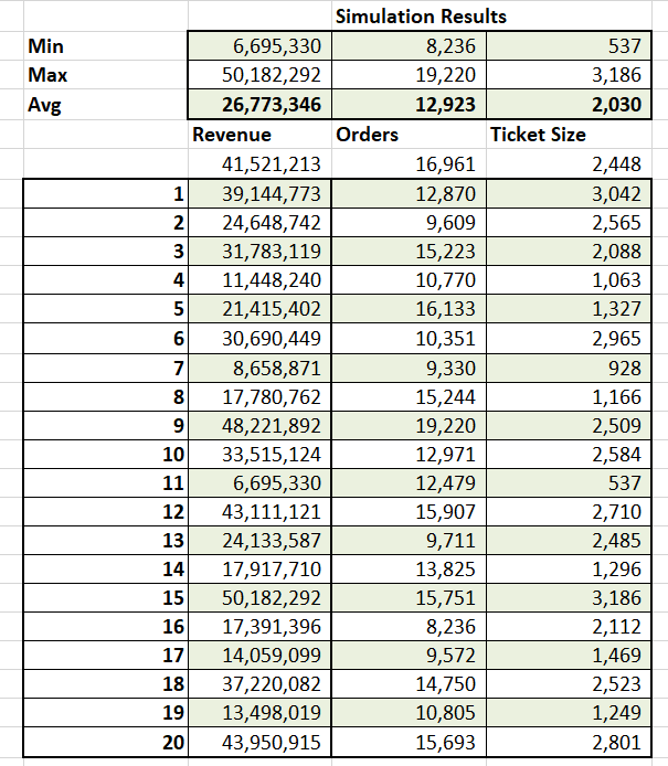
The profile gives you a range for results (minimum and maximum) and the expectation – the averages for revenues, orders and order size based on simulator you have built. The values are volatile because you ran 20 trials. Extend trials to between 500 – 5000 for stability.
Stability is achieved when the averages stop moving around too much and the shift in the average results is in decimal points rather than whole numbers. Depending on the complexity of your model, you may hit stability with 1,000 simulations or you may need 25,000.
How does the Monte Carlo simulation work?
Excel takes the trial number and plugs it into the cell you specified under column input cell. That triggers an update. The update triggers a new random number and a new value. Because it is a data table, Excel stores it for you saving you the manual labor.
Why bother adding Monte Carlo simulations to your financial model?
Remember you wanted to understand the distribution and had no prior data except just industry trends. Well now you do. You have a distribution of results. That can help you answer your questions. More importantly that distribution uses 3 simulated variables.
It also captures the interaction between simulated orders, ticket size and share of traffic based on click through and conversion rates. Switch the distribution, flip the input and try other metrics.
The results will change but the model will remain the same.
Just one qualification
We assumed simulated variables are normally distributed and our sampling (trials) is straight from the distribution. Financial markets need more complex models. Different models for equities, FX and commodities. Different family for interest rates.
Two good questions that were posed privately.
- If you don’t have a mean or standard deviation, where would you get one from?
- Even if you did or do, wouldn’t the distribution average up to the same values? If yes, then why bother, what’s the point?
What do you think?
The first question is easier to answer. Look at industry benchmarks. Look at your financial plan or budgets. Review competitors’ financial disclosures. All else fails, do a google or twitter search. You would be surprised at what pops up.
The second is more difficult and nuanced and will take more time.
Derived results. Let me see if you can figure out the answer with this image. We simulated
- Click through rates
- Landing page conversion rates
- Ticket size
We didn’t simulate orders. But the model still gave us the distribution. Not just the expectations.
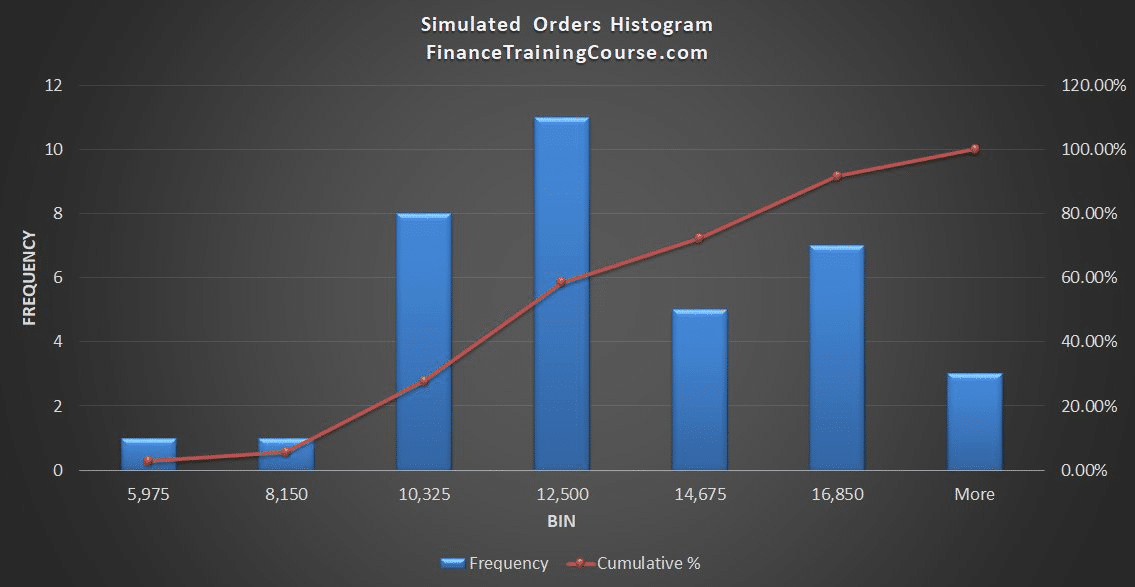
Why does that matter?
Because without an explicit model for relationship between click through, conversion and order size, we built a model for orders. Derived results are the reason why Monte Carlo simulations are such powerful tools for our financial models. They help us frame indirect but relevant results.
You can also answer other questions.
What is the probability that we run short on cash in the next 3 months? The probability that will hit a certain revenue run rate? That chance that we will need another round of funding?
Derived results. All of them.
Which brings us back full circle.
Your simulation is as good as the questions you ask.
Just like the Oracle, from The Matrix. Focus on asking the right questions. Then build the models.