Modelling growth for founders and startups
When building financial models founders often get growth and downside risk wrong.
Our horizons are limited by the standard 5%, 10%, 15% up or down or the more extreme 50%, 75% and 90% up scenarios. While these may work for a single year, it is rare for a business to continue growing for multiple years at extreme growth rates.
Here is a short case study based on live data from Maya’s closet, a team we mentored at Karachi based technology incubator at Nest I/O.
The context is finalizing a growth outlook for 2020, while reviewing news and data in February 2020.
From a timing point of view February 2020 represents an inflection point. Old data and growth rates are no longer a good predictor of future trends because of what a global pandemic is likely to do to networks, logistics and consumer demand. Since the disease and the virus is new, we don’t know how long the pandemic would last and when would be a realistic date for the world to open up.
As the founder, you are seeing bad news across vendors, partners, and customers. Given your historical rate of growth, you are worried about 2020 and 2021. You need a data driven forecast, sans guesswork. Why?
Because you are dependent on your suppliers for just-in-time inventory. If you order too much and orders tank, you are out of pocket for the cost of inventory. If you order too less, it will not be possible to restock inventory given anticipated delays in logistics and supply chain because of pandemic related restrictions on travel and transportation networks.
What is your goal? What is the question you are trying to answer?
You want a data-driven, projected order number for 2020.
If you could get the forecast monthly, that would be terrific. But you would also be happy with an annual figure.
You are aware that any forecast for the next 3 months will be completely wrong given the uncertain situation. But you are lucky to have some operating history, so you dig out 5 years of sales data. Your mentor suggests you organize it by year and month to track seasonality.
Once that is done, you must decide what lens to use to interpret these statistics. Different lenses mean wildly different deductions.
Should you just look at annualized growth? Month-on-month (MoM) growth? Or should you look at seasonal trends?
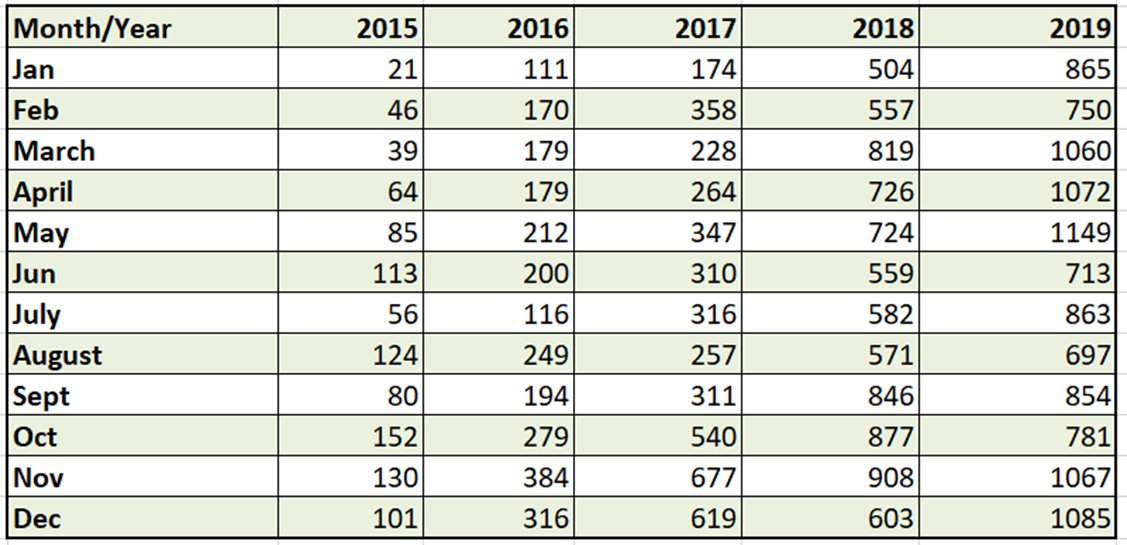
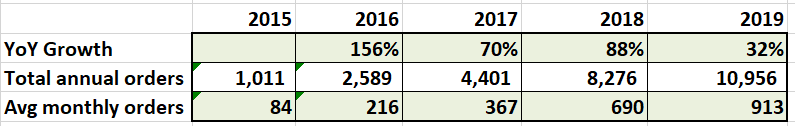
A first pass gives you a basic trend. Growth has been slowing down every year as you step up sales, order volumes and revenues.
In 2019, you grew a healthy 32%. What will be the growth rate in 2020 and 2021?
Maybe the news right now is just a bad scare? May be the restrictions are temporary and will be over by the time we get to summer? Or, maybe, just maybe we are looking at a global pandemic?
On the bright side with brick and mortar stores closed, shut down or locked away, demand for online shopping and curated services such as the ones you provide may rise.
One thing you are sure about. Even if this was a normal year, growth in 2020 is going to be lower than 32%. Given the trend so far, likely to be somewhere between 20% and 10%.
Why?
Because it is more difficult to grow 11,000 orders by 25% than it is to grow 4,500 orders by 50%.
While the absolute magnitude of orders is similar (2,750 vs 2,250), there is a higher chance of hitting capacity constraints with 13,250 orders than there is with 6,750 orders.
Step functions
What do we know so far in terms of context?
- We are not going to grow at 156% a year, year on year, forever.
- We grew by 32% last year. We will likely grow between 10% and 15% this year, if this year was a normal year.
- Growth will slow down. For some it will slow down faster.
- In our specific case, we have been organically bootstrapped all the way. We are constrained by capital.
- We could be constrained by complexity, bandwidth barrier or even worse, regulatory challenges.
- This year is not going to be a normal year. We don’t know if its going to be good or bad.
These constraints are a result of step functions. Step functions represent capital, capacity, or resource constraints. They create discontinuities in your growth curve. When you hit a step function it is like hitting a wall.
You can order inventory for a year but where will you store it? Who will pack it, ship it, answer customer queries, and manage returns and refunds?
Growing businesses hit step functions. Find out where the next step function is or will be for your business. We do not have infinite capacity, bandwidth, or resources. Estimate maximum threshold, and then factor in the cost of upgrading team, infrastructure, and resource pool.
Taking the monthly lens
If you take the monthly lens, the figures look a little different.
January is a good month. It is a slower month than December but every year in January spill over orders from December lead to a growth spike specific to January.
Growth and order wise, November to January tend to be the strongest month of the year and represent peak season for our business.
Followed by March, April and May.
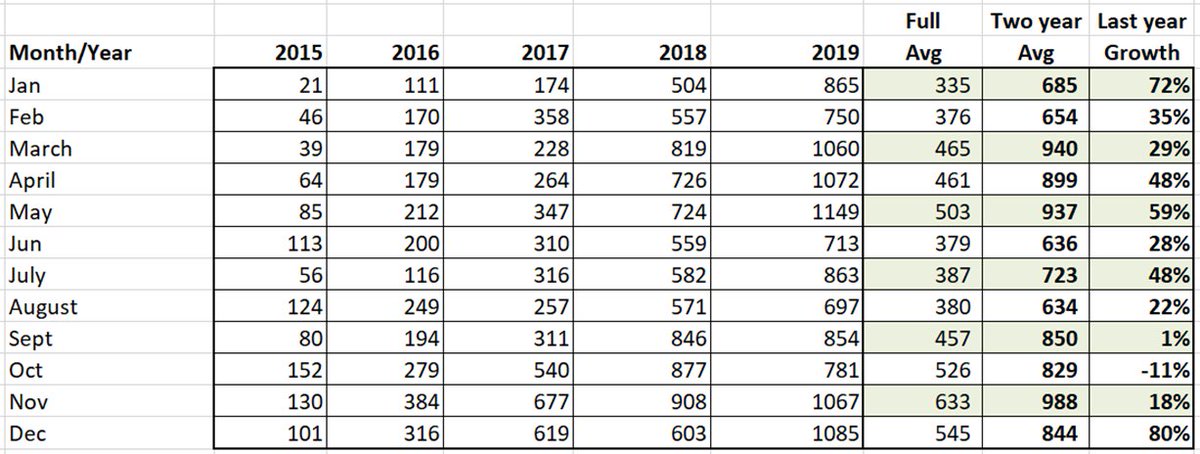
We calculate the 5-year average first but don’t think it’s relevant since relative order volumes on a month-on-month basis are very different between the first year of the data set and the last year.
We try again with the last two years of orders (2018 and 2019) and the average is better than the 5-year average but we are not sure if this is the right approach. Should we use the full data set? Should we use the most relevant and recent trend? Which one is more appropriate?
All the availability of data has done is create confusion. We are still not sure how to get to an answer.
Perhaps because we are not asking the right question? What is the question we are trying to answer?
With zero growth, will we complete 11,000 orders in 2020.
If we grow at 30%, we will process 14,300 orders. With 10% growth, we will do 12,100 orders.
The questions we ask ourselves are the following:
Which one of these scenarios is more likely than others?
How can the data above help us in answering this question?
What is the best way of modeling and answering these questions?
Possible Solutions. Model A. Growth with absolute values
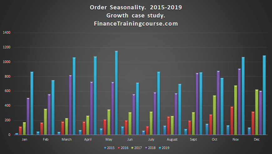
You call your mentor again. He says, send over the dataset. An hour later he sends you the following graphs. A nice colorful representation of your orders by month.
You already had the numbers, but he follows up with something different.
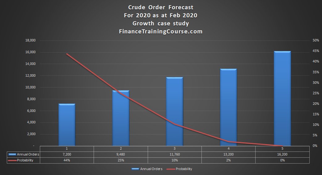
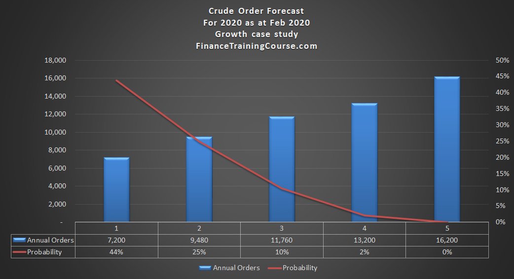
A probability weighted forecast of your annual orders for 2020.
His short note says.
“This is for business and usual. We are all truly #$%@*&. It not going to be business as usual. Order less. That is the best I can do right now. And if you want more accuracy, either come over or give me time.”
He also sends something called a histogram that he says is the basis for the order probability calculator above. You now know you should have paid more attention the last time he walked you through this concept.
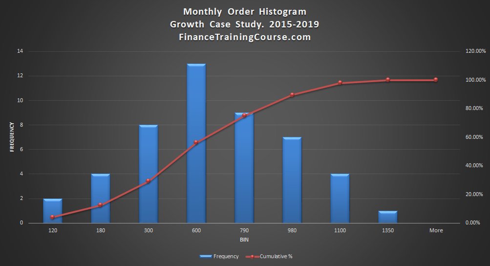
The histogram is just a different representation of the orders data.
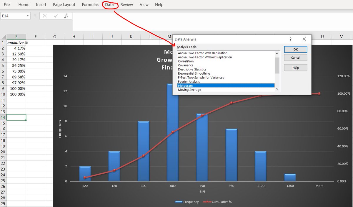
All we have done is sorted the orders, bucketed them, and plotted the buckets. That is where the distribution comes from. Excel will do this for you with the histogram tool under Data Analysis.
In your case, the histogram tool shows you the plot of the distribution of monthly orders from the last 5 years. And an associated cumulative probability plot based on that distribution.
What is the most likely number of future orders for a given month? 600. The probability of a monthly order volume of over 1101 orders or higher? Low. The odds of seeing 600 or more orders in a given month? Even. We read the above from the chart below.

But where did the order probability calculator came from? We used a really crude/terrible assumption:
We assumed that we would see the same monthly order across 12 months of 2020 with the same probability. 600 monthly orders becomes 7,200 annual orders.
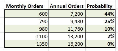
The calculator is the just the plot of the table above.
My statistics professor will have me shot for even suggesting this as a model. To the untrained eye, however, it looks legit and impressive. And yet, it’s completely wrong.
Model B. On the merits of relative change
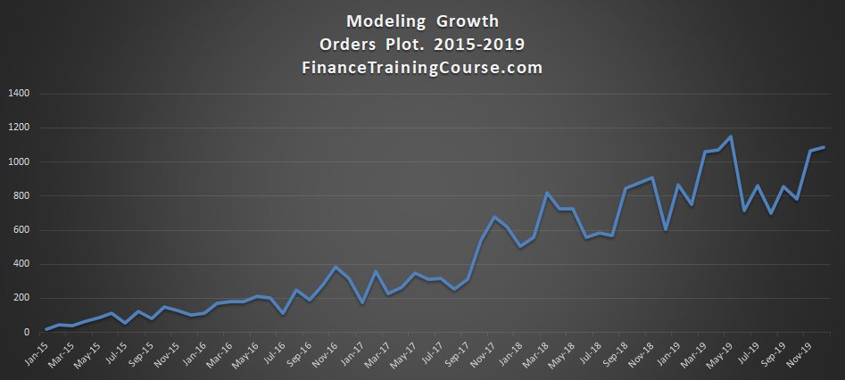
This is what our order flow dataset looks like. From Jan 2015 to Dec 2019. You can see the seasonality impact and the trend in the graph below.
We can’t use 2015 for 2020 forecast data because it’s too low when compared with the most recent year figures.
To get around this issue, here is the relative-percentage-change plot for the same data set. The trend is now levelled. You can now use the 2015 and 2016 data set that we had to put aside in our analysis initially.
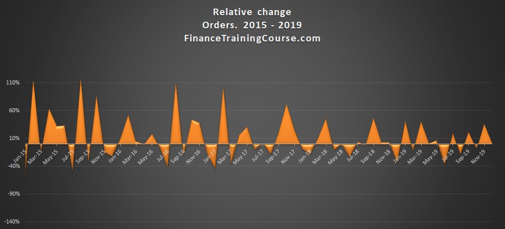
Because of the low base size there is higher volatility in initial years but because of relative change, we can still use it in our forecast.
We can now use this data set to plot a new histogram. One that uses relative percentage change in orders rather than absolute order values.
Meet the relative change histogram showing distribution of percentage changes across 4 full years of data. The most common and likely monthly change is a drop of -10%.
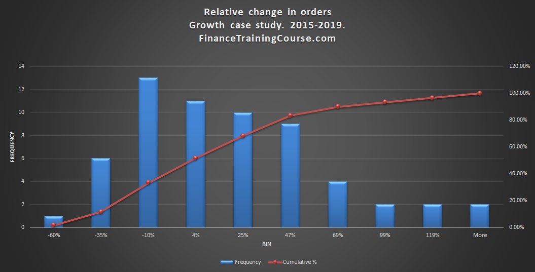
The probability of seeing a minimum or lower growth month is higher than the probability of seeing 5%+ mom growth.
Remember. These are normal operating conditions. In February 2020, we are going through something completely unprecedented in recent history. Conditions the world saw over a hundred years ago.
If the probability of seeing 4% or lower (including negative) growth is 51% under normal conditions, what would the probability be amidst a global pandemic?
The relative change plot below shows 1/3 of your data is ‘down months’. Months where order volume fell compared to the previous month volume. Intuitively speaking we would expect a higher proportion of down month in a global pandemic.
The most likely answer to the question posed above is higher than 51%.

Two big benefits of using the relative change model, model B compared to model A.
- One. We can use more available data and we are no longer limited by size of our order book in earlier months, where order volumes were low.
- Two. We now also have a range and frequency of relative changes, which is useful in setting expectations.
Question: Will March 2020 be a down month. Yes.
33% chance that we see a drop between 10% to 60% of orders in March 2020 using normal dataset and conditions.
Possibly higher since we are in pandemic mode.
Will April and May 2020 also be down months? Yes, but with increasingly lower probabilities.
Why? Because probabilities multiply when we use “and”.
Will March and April and May be down months? If the probability of a single down month is 33%, probability of 3 down months in a row would be lower than 33%. How low? About 3.3%.
This holds true even after making adjustment for pandemic mode.
This was the issue with our earlier analysis in Model A. The crude assumption that was incorrect. We used it to get a crude answer, but we knew the answer was going to be off going in. Why? Because we did not factor in the impact, the probability that orders will stay at the same level month on month. We assumed they would.
How do we put this to work? How do we jump from month to years?
Feb 2020 orders data has just come in at 958 orders. Jan ’20 was 703. Dec ’19, 1085.
Based on everything we have shared so far, what do you think March and April figures are likely to be?
Remember sometimes the best way to learn something new is to start with the wrong models.
Forecasting Monthly orders for March 2020
Our model is based on historical data from a normal world.
In Feb ’20, we are in an abnormal world. Normal rules have been put on hold.
Under the normal world dataset / histogram, we had even chances of seeing 4% or less, 4% or more growth.
In the pre-pandemic stage in Feb 2020 the safe bet is negative growth.

How much negative?
Between the -10% and -35% for March 2020.
But what we can do is figure a fix for the rest of the year. What is our outlook for the remaining year?
At -10% to -35% reduction in orders we estimate between 622 and 705 orders for March.
Giving us total Q1 orders between 2,284 and 2,366.
Historically from the same data set we know the relationship between Q1 orders and (Q2+Q3+Q4) orders.
It ranges between 3x to 4x.
Assuming a down year, we go with 3x.
Our expected order range for full year 2020 is 9,135 – 9,1465.
We have our number. Sounds like pseudo-science but it is more credible than a shot in the dark. We have used our data set and a simple excel tool to make an educated guess.
The same approach, model and design can be used to get to sales forecast for a given month or a given year using historical sales data. Update the same when new data is available. Assuming your sales team can deliver on the same magic they had working for them in the past.
What did 2020 look like for our friendly ecommerce startup?
When we started with our analysis we had three possible scenarios in mind.
A low or zero growth business as usual scenario. If this was a normal year and the trend of slowly reducing growth had continued, expected orders would have grown but at a slightly slower or lower rate.
An explosive growth year. Given the wide pick up received across categories in online shopping as lock downs rolled across regions, this may be a valid and likely scenario
A catastrophic decline. Given logistical and supply chain constraints, while customer interest went up, the store had no inventory to process orders and fulfill demand.
What scenario do you think was likely sitting Feb 2020? Which one do you think finally came to pass?
March was down 38%. But they still managed to grow a respectable 15% year on year compared to their 2019 results.
Their actual (Q2+Q3+Q4)/Q1 ratio? 4.5x compared to the expected 3x.
They reacted faster than others.
A quick summary
- Can’t keep on growing at 156% yoy. Growth slows down.
- Have sales/order data use relative change vs absolute values to predict/forecast future change.
- Growth modeling comes in many flavors. Simple to complex. Make sure you have your basics right.
Conclusion. The 6 common mistakes in setting growth assumptions
The 6 common mistakes to remember while setting growth assumptions in financial models.
Lesson one. Growth is never free.
Need a new warehouse for higher inventory. Also need customer service resources, faster servers and infrastructure for load.
Marketing dollars and capital for financing receivables and current assets. Growth in expenses often leads revenue growth.
Lesson two. Step functions.
Your current capacity has a threshold. When you cross it, you need to upgrade infrastructer.
Modeling step functions in Excel is hard because it breaks the flow of the model. Updating and maintaining step functions is also hard for the same reason.
Lesson three. Downward sloping, caps, and floors.
Growth slows down over time.
It is capped by capital, capacity, and market conditions. It also has a floor often set as a small multiple of regional or national growth numbers.
Lesson four. Consolidation.
Most growth explosion are lucky accidents. When we get it right, the market doesn’t give us time to sit back, process and think through implications of growth. We react to growth and often make decision that may work in the short term but need to be rectified before they do serious damage.
Consolidation is when we take a break, think throw and fix what is broken so that we can continue to grow.
Consolidation often leads to negative growth. We shed baggage, fix processes, write off balances and relationships. Consolidation is a requirement for continuing growth without killing ourselves and our businesses in the process.
When a team or a business has been growing at a fast clip for multiple years, consolidation is inevitable. Budget for it, plan for it.
Lesson five. Data
Look at historical trends. If you do not have history look at industry metrics.
While you may disrupt some of them, you are married to most of them and will ultimately be pulled down towards them.
Just like gravity. And no, while we may feel like it, no one is smarter than the incumbents.
And yet in instances like the pandemic, be prepared to walk away from historical data and build a new model from zero.
Lesson six. Replacement products.
Products have a shelf life ranging from a few months to a few years. To continue growing you need to invest in a new product pipeline. Without the pipeline, your growth will stall.
Product R&D is expensive and often hit or miss. Budget for it.