Here is an abbreviated partial solved solution to the practice exam question posed earlier. The practice exam question was used in the Derivatives Pricing course taught to MBA students earlier in August 2012. The solution is presented in two parts. The first part of the solution focuses on the bootstrapping forward curve and the zero curve part of the exam. The second part of the solution walks through the actual IRS pricing exercise. This post covers the first partial solution.
The practice exam question had three parts and hence the solution to the practice test question will also be presented in three parts. Before you proceed further please take a quick look at our free interest rate swaps pricing guide. We will only present the basic outputs from the solved solution sheet. You will need to review the interest rate swaps pricing study note to actually build the sheet yourself on your laptop.
A review of the solution approach
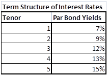
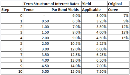
Practice Test Part I dealt with the building and plotting the Zero and Forward curve using the data given and the bootstrapping approach applied on the given interest rate yield curve given below. The original yield curve was a 5 step curve that gave 5 annualized rates for 5 years.
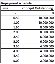
Practice Test Part II dealt with using the given zero and forward curves to price an Interest Rate Swap (IRS) and calculate the swap rate. The trick was extending the original curve to the new 10 step, semi annual yield curve implied by the 10 step notional amortization schedule given below.
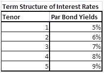
Practice Test Part III dealt with marking to market (MTMing) the interest rate swap for an updated curve a few months later. Once again the trick is to extend the 5 step curve to a 10 step semi-annual curve which can then be used for pricing the interest rate swap.
Solution Part I – Building the Forward Curve
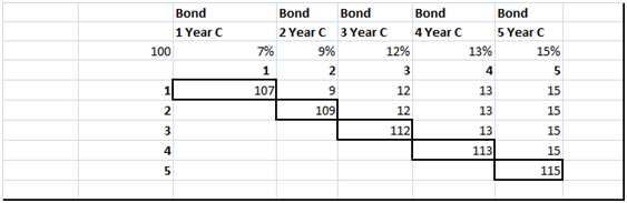
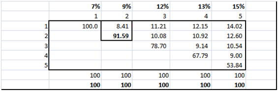
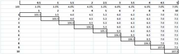
The first step is to break the individual bonds down to their annual cash flows and treat each cash flow as an individual zero coupon bond as explained in the interest rate swap pricing study guide. The output from the first forward curve building step is shown below
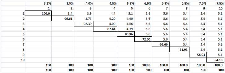
The second step is to use the individual zero coupon cash flows to boot strap the present value of the principal cash flow at maturity for each of the par bonds as explained in the interest rate swap pricing study guide. The output from the boot strapping step is shown below.
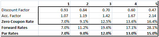
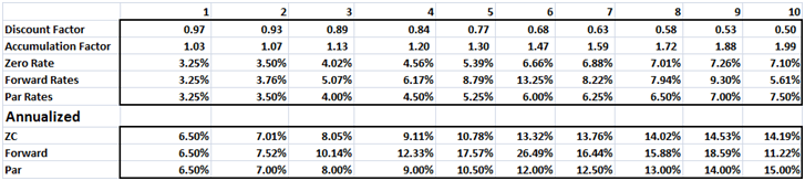
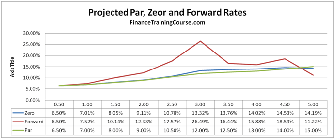
The third step is to apply the zero curve and forward curve formula to calculate the relevant zero and forward rates from the table above. As explained in the interest rate swap pricing study note. The output from the zero and forward rate calculation step is shown below.
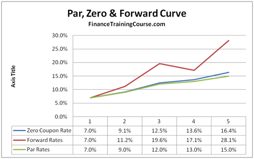
The final and fourth step is to plot the Par, Forward and Zero rates in the required graphical format using MS Excel built in graphic tools.
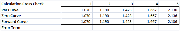
Most students make it to this stage without any incident. Some, however, apply the wrong formula and end up with inconsistent results. If you are not happy with the results just apply a simple calculation cross check. If you calculate the relevant accumulation factors for each given year using your calculated Par, Zero and Forward curves they should all result in the same values as shown below.
The Par Curve Accumulation factor was already calculated above. For the Zero curve the accumulation factor is (1 + zero rate) raised to (compounding period). The accumulation factor for the forward curve is a similarly recursive calculation. Calculate the accumulation factor using the forward curve for the first year. Then use that in your calculation for calculating the accumulation factor using the forward curve for the second year.
If you see a value in the error term row, you have made a mistake in the calculations above. Review and check them.
We have now successfully completed the first part of the test question. We now move on to part II.
Solution Part II – Extending the Forward Curve
The second part of the question requires us to use the interest rate yield curve above to price a 10 step, semiannual interest rate swap. And this is where confusion reigned supreme.
Step One – Interpolated semiannual yields
We first need to break the original annual yields to maturity down into interpolated semiannual yields as shown below
Then using the same sequence of steps above we break the new implied semiannual bonds down to their zero coupon components, boot strap the curve, calculate the rates and plot the graphs.
Step Two – Zero Coupon Bonds
Step Three – Bootstrapped Discounted Cash Flows for Zeros
Step Four – Periodic and Annualized Par, Zero and Forward Rates
Common Mistakes in Part II of the Test Exam
The most common mistakes that killed points for students in the second part of the practice test and exam questions were:
a) Not calculating the interpolated semiannual yields and using the original 5 annualized yield to price the 10 step interest rate swap
b) As a result of (a) above building a 5 x 5 or a 5 x 10 grid versus a 10 x 10 grid as shows in step two and step three above
c) Using annual rates rather than period rates in the 5 x 10 and 10 x 10 grid. Periodic rates are annualized rates divided by 2 since the coupon on the underlying loan is paid semi annually
d) Using periodic rates but then not annualizing them before using them in the IRS pricing later on in Part III of the practice test exam.
The correct solution and required graphical presentation if you didn’t suffer from mistake (a), (b), (c) and (d) above would look like this:
We continue our coverage of this exam question in our next post.
Comments are closed.