So far in the portfolio optimization course our focus has been on single dimension analytics. With both risk and performance we have only looked at one metric at a time. While our Solver models have worked with multiple constraints, the constraints themselves have focused on singular relationships. With the market index (Beta), excess return with respect to the market return (Alpha), worst case single day loss (value at risk), traded volume and number of exit days (liquidity) and holding period return (return). It is now time to introduce something slightly off the beaten track. Say hello to Skewness preference or higher order portfolio models.
Can we use an optimization model to shift the return distribution. The question we are trying to answer is “Can an optimization model increase the probability of positive return”. For random, normally distributed returns, there would be roughly an even chance of seeing a positive or negative return on a given day. An effective portfolio management tool should be able to improve the odds.
Can we actually shift the distribution using our optimization tools? More importantly in addition to all the other metrics discussed so far, can the return distribution from our portfolio give us a broader performance metric that can be used to evaluate portfolio performance.
Let’s compare two return strategies.
Our first strategy relies on a random choice. We will use a coin toss to decide whether we are going to buy or sell today. To keep our model simple we will work with a single security. Every morning we will toss a coin and decide what our plan of action for the day would be. If the toss reveals a head, we will buy; if it reveals a tail, we will sell.
This will serve as our benchmark for performance evaluation. It is not completely random since we have some input in security selection and we can pick the right stock and bias the results to some extent. The buy and sell decision and the timing of that decision is random. For our first experiment we pick a security that is expected to generate an average daily return of zero and a daily standard deviation of 1%. And we assume that the expected returns on this security will be distributed as close to the normal distribution as possible. What do we expect to see when we plot the portfolio returns generated from this strategy?
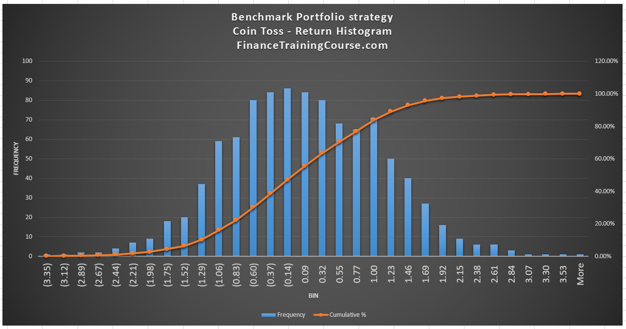
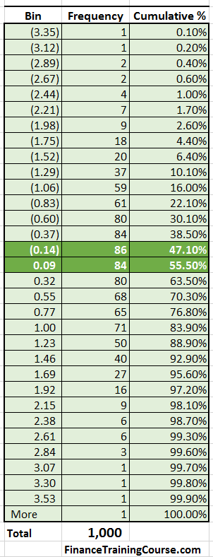
You can clearly see that the midpoint of the return distribution lies between daily returns of (0.14%) and 0.09%. Essentially very close to zero. More importantly when we examine the data set underlying the graph we see that there is roughly a 50% chance of seeing a positive return. And a 47% probability of seeing a negative return with this strategy.
This performance will now serve as a benchmark. If you are an effective investment, portfolio or fund manager you should be able to beat this return. If your investment allocation framework, model, approach or philosophy works you must be able to outperform a random coin toss.
A non random strategy – Maximizing Alpha
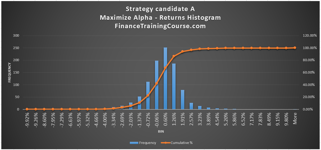
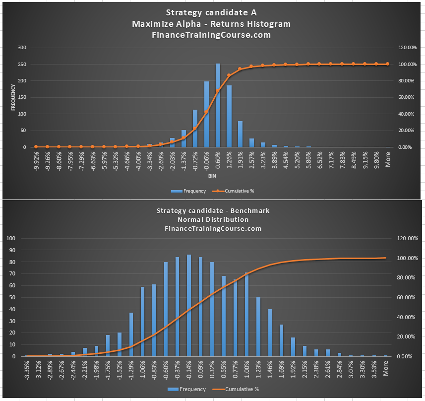
Compare this with our second strategy – a non-random one. We have used this strategy before within our portfolio optimization sessions. We create a portfolio that maximizes Alpha over a given index. For ease of comparison we produce the two histogram tables from the two returns distributions side by side.
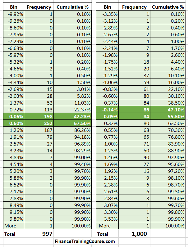
Compared to our original random strategy a few things are immediately visible. The range of returns has increased – from plus minus 3% to plus minus 9%. The center of the distribution has shifted. The probability of receiving a positive return has increased. The probability of recording a negative return has also decreased. The new optimized distribution is a lot more compressed compared to the random one.
Together with the data set above and the histogram comparison below we can see the impact security selection and optimization has made on our portfolio returns.
The question is that if by just focusing on performance metrics we can create an impact in the underlying return series, can we create a bigger impact by specifically focusing on right shifting (to the positive) the distribution? Our most recent portfolio returns candidate has a higher chance of seeing a positive return on a daily basis and a slightly lower chance of recording a negative return. Can we push these numbers higher? If we do what impact does it have on other core portfolio performance metrics?
Introducing Skewness preference
Skewness is the average cube deviation from the mean, divided by the cube of the standard deviation. Positive for positively skewed, negative for negative skewed, zero for symmetry. Our interest and objective is to push the distribution to the right, into the positive skewed territory to improve the odds of seeing higher, positive returns.
Cindy Tsai at Morning Star wrote an interesting paper on the new Mean Variance Optimization frontier in 2011. An optimization frontier that also looks at higher moments such as portfolio Skewness (third moment) and Kurtosis (fourth moment). The concept is fairly simple. Emphasizing positive skewness in portfolio selection would increase the probability of positive returns. We would literally shift the distribution to the right. Hence the term skewness preference or higher moment portfolio models.
When we apply the concept to our data set and portfolio we see some interesting trends. Calculating and adding a Skewness constraint to our portfolio returns and including that in our solver models clearly shifts the returns distribution center to the right. To calculate skewness, simply use the Excel function SKEW. Calculate skewness for the portfolio return series and then add a condition specifying the minimum acceptable portfolio skewness to your Excel solver model. Run the solver model as before and compare portfolio metrics as described earlier in this course.
How significant is the impact? Let’s take a look.
The next panel presents three different returns distributions. The top and bottom panels have were generated after adding a skewness preference constraint to our portfolio optimization solver model. The panel in the middle is the original strategy without skewness preference in place.
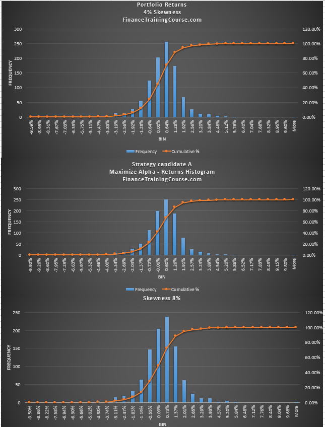
Can you notice the difference? At first glance they all look the same.
Take a look at the center of the distribution. In both the top and bottom panels with the skewness constraint, the return distribution has shifted. Compared to the original strategy, there is now a significantly higher chance of recording a positive return. Of the 1000 days of data, more than 700 days now lead to a positive return in the two panels with skewness preference. Compare this with the original 576/1000 without the skewness preference in place.
Here is a closeup of the bottom two panels for a quick comparison.
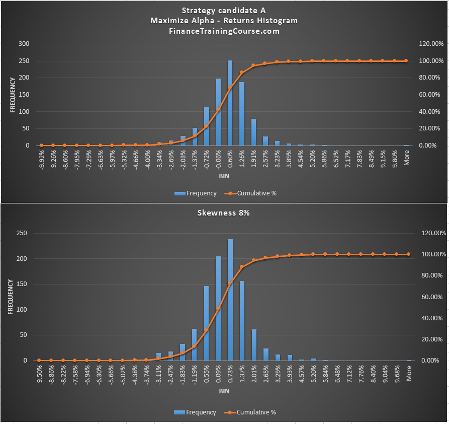
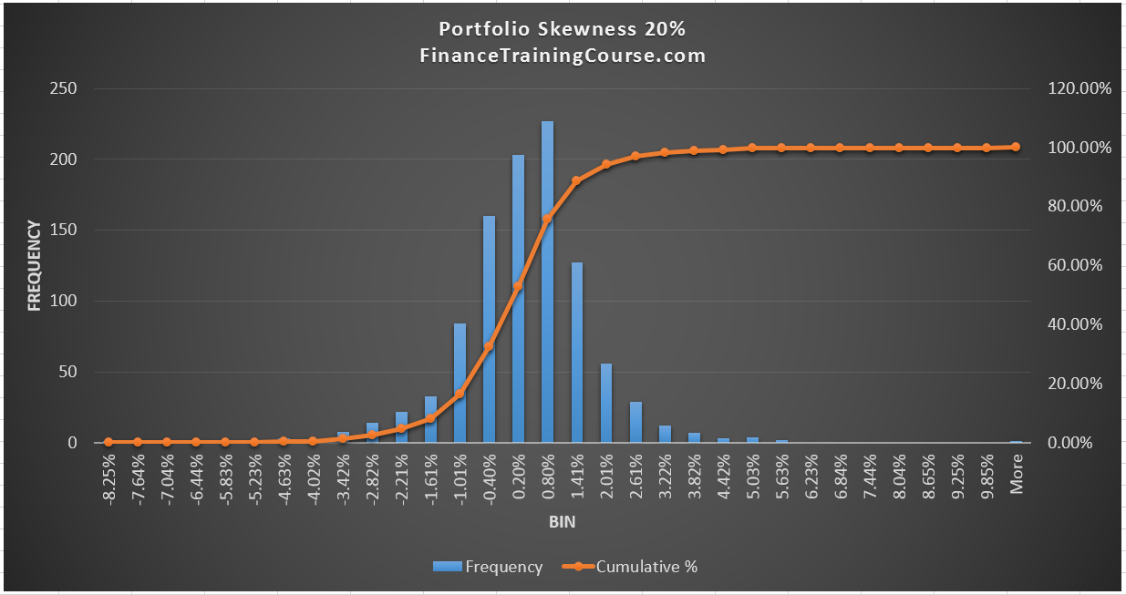
There is a cost though. We drop a few basis points of returns and add a few basis points of volatility. A better distribution with a higher likelihood of a positive payoff but with slightly lower returns and slightly higher volatility. Does this mean that more skewness is better. Not necessarily. For our data set and our portfolio, the objective was to shift more returns to the right. We achieve that with 4%. As we increase the preference first to 8% and then to 20%, the number of days with positive returns begins to fall again.
The next image and table show a quick summary of the results we have discussed so far.
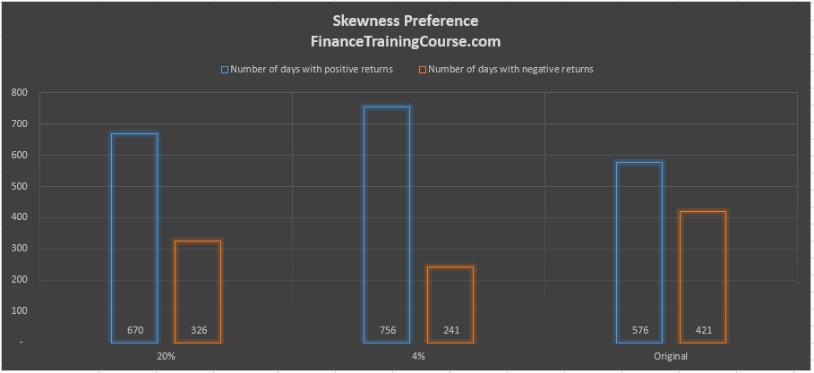
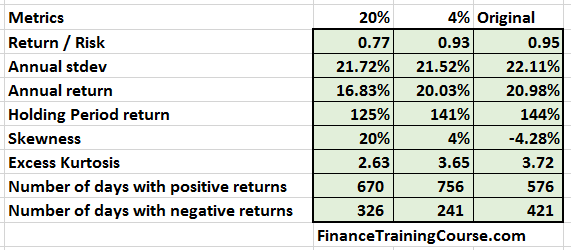
Our original max Alpha strategy without skewness preference had a negative skewness of 4.28%. The number of days with a positive return in that strategy was 576. With a minor tweak to our optimization model, we dropped almost a full percentage of expected annual return, reduced the standard deviation by half a percent but were able to improve the number of days with a positive return to 756. For the small price we paid in terms of the change in return per unit of risk metric, the improvement in the return distribution is significant.
Now that we have tackled skewness, as a takehome assignment, repeat the same process with Kurtosis. How would you describe the value addition from adding an additional constraint?
References and additional reading
- Cindy Tsai, The real world is not normal, 2011, Morning Star.
- Xiong, James X. and Idzorek, Thomas, The Impact of Skewness and Fat Tails on the Asset Allocation Decision (April, 11 2011). Financial Analysts Journal, Vol. 67, No. 2, 2011. Xiong and Idzorek (2011)