On day one of our course on portfolio management we introduced basic concepts and challenges of portfolio management. We introduced the securities universe we are planning to use for our five day workshop. On day two we begin building our Excel portfolio management worksheet.
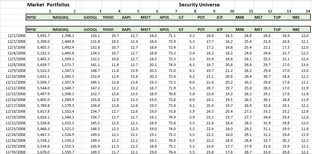
We begin with the raw securities price data set. You can download the data set here.
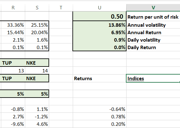
And end with a return series sheet with individual security and portfolio metrics:

Once the Excel portfolio management spreadsheet is completed we will explore a number of portfolio optimization challenges in the following posts. These include:
- Beating the performance of a given benchmark index. We will explore matching and exceeding the performance of NYSE (DJIA) as well as NASDAQ (Technology and small cap stocks).
- Optimizing risk and return for a portfolio limited to just equities, as well as bonds and commodities.
- Investigating the optimal mix of portfolio Alpha and portfolio Beta. We are also interested in what investigating Alpha and Beta heavy strategies reveal about market neutral fund performance.
- When we introduce a bond, currency and commodity indexes we would be interested in seeing the impact of additional diversification these new asset classes bring to our portfolio.
- Setting risk limits as well as introducing the concept of Kelly’s criterion for right sizing bets
- Exploring alpha cyclicality and the possibility of building a trading algorithm around it that generates both buy and sell signals.
Please download the data set in Excel if you haven’t done so as yet. You should check to ensure that you have price series for 2 market index and 15 equity securities. In the next few steps, we aim to complete all of the following with our raw portfolio data set.
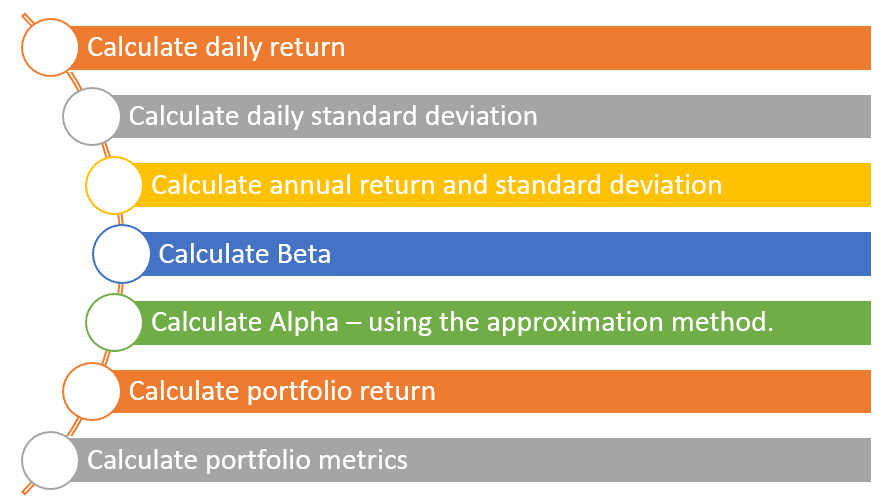
1. Calculate daily portfolio return and average daily return.
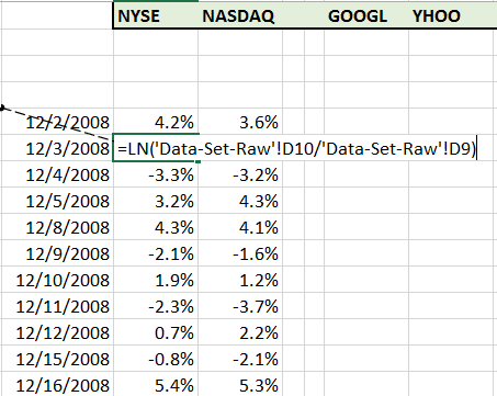
Begin by calculating the daily return series for the two market index – NYSE and NASDAQ. Rather than using (New Price – Old Price)/Old Price or (P1 – P0)/P0 we use the natural log function to calculate the daily percentage change in price as shown below. The end result is approximately the same and it will make working with a few assumptions easier in the latter half of this course.
You can do this on the same tab as raw data or create a new tab titled return to add more structure to your spreadsheet. Repeat this for both NYSE and NASDAQ and make sure you calculate it across the entire data set (1851 rows).
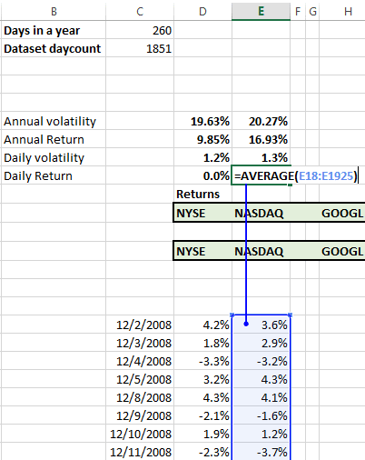
Once you have calculated the daily return series, calculate the average daily return using the Excel AVERAGE function as shown below for both NYSE and NASDAQ.
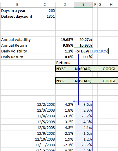
2. Calculate daily standard deviation
Calculate the daily standard deviation by using the Excel STDEV function for both NYSE and NASDAQ.
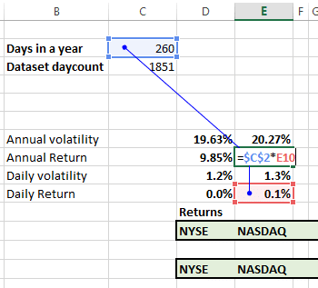
3. Calculate annual return and standard deviation
Annual return is simply the number of trading days in a year multiplied by the average daily return.
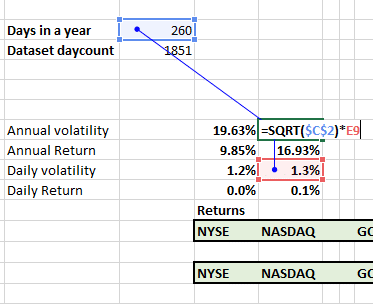
Annual standard deviation is the daily standard deviation multiplied by the square root of trading days in a year.
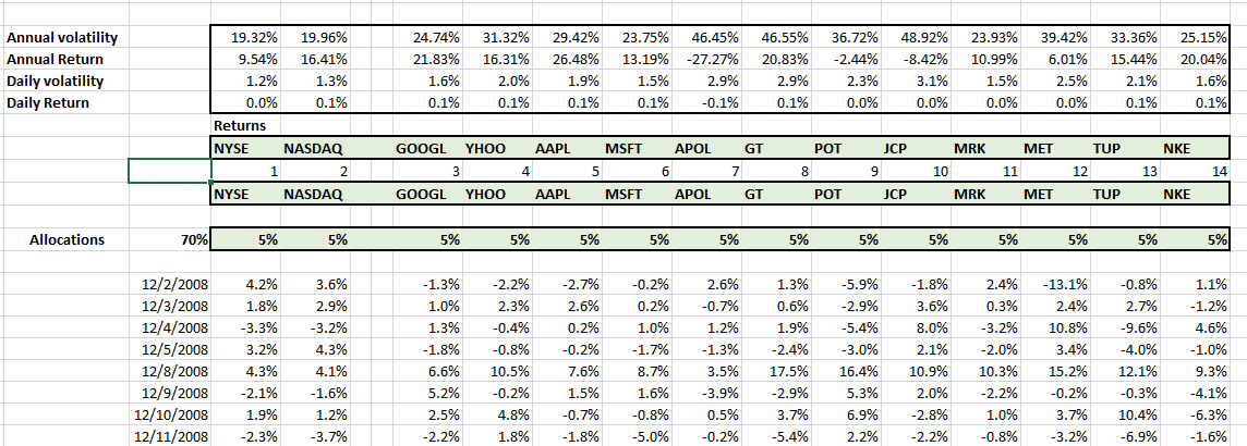
Now that you have calculated the basic metrics for the NYSE and NASDAQ repeat the calculations for the other 15 securities in the universe till you end up with the basic metrics for all the securities.
See Portfolio risk metrics- volatility for a detailed treatment of the calculations presented above.
4. Calculate portfolio returns
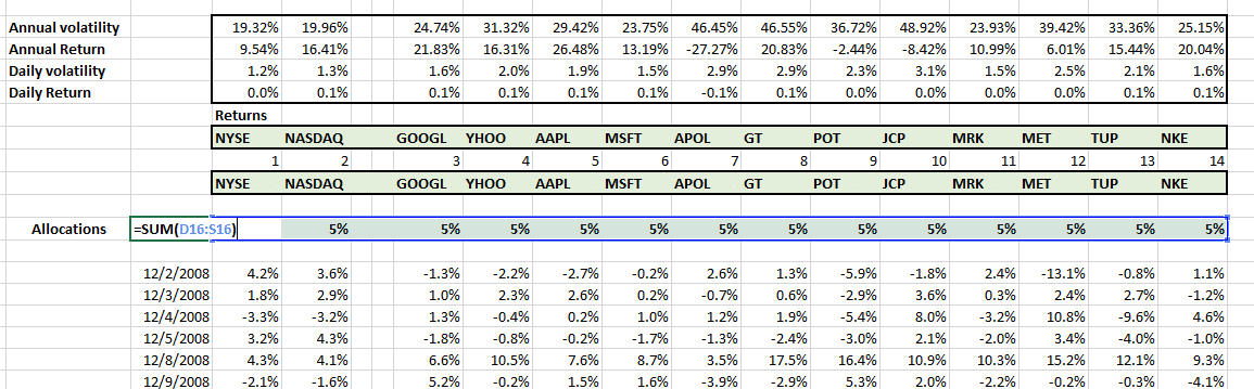
Now that we have everything in place, we are ready to calculate portfolio returns. We first need to add security allocations. Do that by plugging a placeholder value of 5% across all securities in the empty row between daily returns series and the security tickers. We put the placeholder values in place for now but these will be replaced when we run our optimization cycle using Excel solver.
Sum up the allocation so that we have one cell pointing to the total amount allocated for the portfolio. We can use this as a constraint to control full investment as well as leverage in later models.
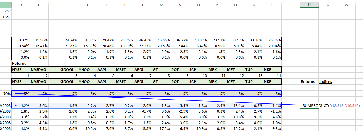
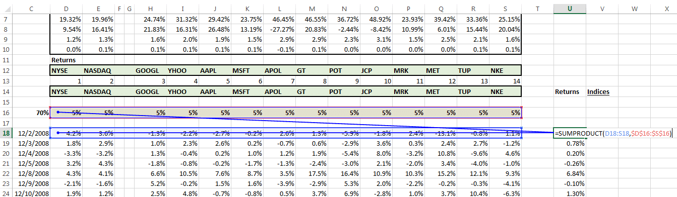
With the allocation in place, we calculate portfolio returns by using the Excel SUMPRODUCT function. The SUMPRODUCT function multiplies two vectors. The portfolio allocation vector (the 5% placeholder values) with the daily security return series to calculate the portfolio return for a given day. Once we have the value for a single day we just need to copy and paste the formula across all days to generate the series for the full data set.
Don’t forget to anchor and lock the portfolio allocation reference before you cut and paste the formula.
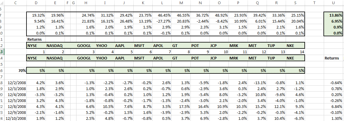
We have the portfolio return series. Go ahead and calculate the portfolio daily return, portfolio daily volatility, annual return and annual volatility figures. You can just copy and paste the formula from any of the security columns to the portfolio column.
Setting up Solver
At this point we have everything we need to do an initial run of Solver to find out the optimal portfolio using the current universe of securities. Given our current set of metrics we can either maximize return or minimize risk. Alternatively we can pick one for the objective function and restrict the other using a model constraint. Another variation is to calculate a single ratio such as return per unit of risk and maximize that subject to additional constraints.
We opt for return per unit of risk.
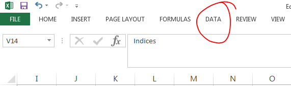
To load up Solver, you are going to need a version of Excel professional. In the Excel menu bar, first pick Data
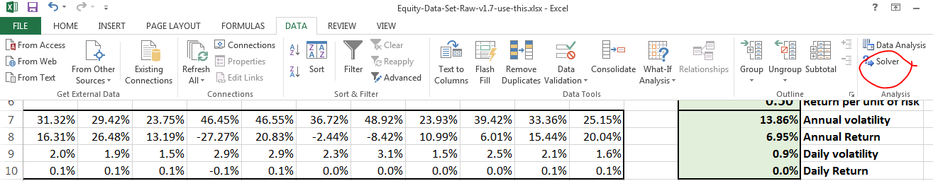
Then pick Solver.
In the Solver setup screen, select return per unit of risk as your objective function and pick maximize.
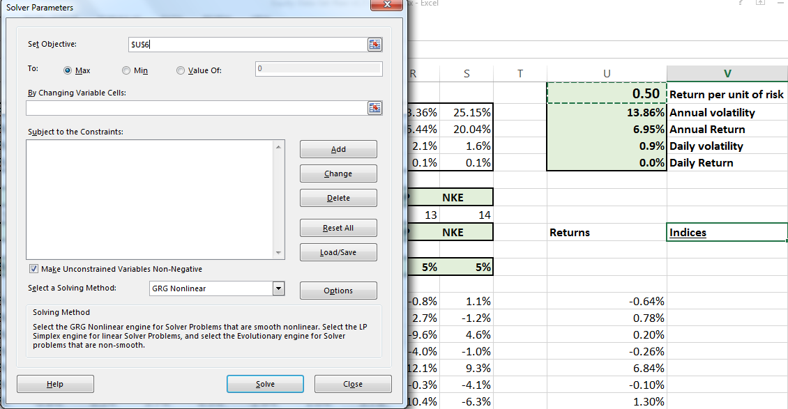
Then under By Changing Variable Cells pick the entire security allocation row we had defined earlier.

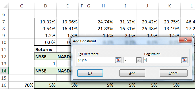
For our initial EXCEL portfolio management model we will add a single constraint which would lead to full investment and that is the sum of portfolio allocation should equal 1. We should be fully invested for the purpose of this optimization.
Just press OK, then press Solve and watch. The model should work. It isn’t complete but given what we have fed it so far, it will generate an optimal portfolio for the setting it was configured to solve.
See if you can identify the part that we need to fix and the problem it is causing. In our next lesson we cover the difference between Alpha and Beta.
Like this post – check out the new book – Portfolio Optimization Models in Excel, 3rd Edition – 307 pages, Excel spreadsheet templates and data set included.
xProduct()