This post provides a step-by-step walkthrough for calculating PFE for IRS using HJM. Potential future credit exposure (PFE) measures counterparty default risk, i.e. the risk that the counterparty to the transaction will be unable to deliver on their obligations thus adversely affecting the entity. To monitor and mitigate these risks, PFE are assessed and limits are set by an entity.
For a general overview of the methodology employed you may consider reviewing the following post from our archives first:
It presents the approach in a stylized form without considering the change in term structure over time or the discounting for time value of money.
This current walkthrough of the calculating PFE for IRS using HJM plugs in the missing pieces, i.e. the interest rate model that generates future term structures, the pricing mechanism that discounts future cash flows and the random simulator that generates multiple scenarios to build a possible frequency distribution of PFE values. It begins by using a multifactor no-arbitrage interest rate model, in particular the Heath Jarrow Merton (HJM) interest rate model, to determine forward rate term structures at each future time step, in this case each leg of the IRS, from issue until maturity. The HJM model applies a Brownian motion, random shocks, to the factors that explain the volatility function of the forward rates. The factors themselves are derived after conducting a Principle Component Analysis (PCA) on the forward rates implicit in the observed market rate term structure used.
For a given simulation run, forward rates determined by the HJM model are used to derive zero curves. These are then used to price the IRS (i.e. calculate the discounted cash flows of the swap) at issue and at each subsequent leg of the transaction. This may be done from the perspective of either counterparty to the transaction. The maximum price across the legs over the lifetime of the IRS is the potential future credit exposure (PFE) for a given counterparty.
The process is repeated for several simulation runs, to obtain a distribution for the simulated PFE. The maximum simulated PFE across all runs is the worst case PFE. However, based on an entity’s risk appetite and tolerance levels, lower exposure levels based on agreed upon confidence levels may be used to set PFE limits. The ratio of the selected PFE to the effective notional amount gives the credit conversion factor for the IRS.
A summary of the process is given below:
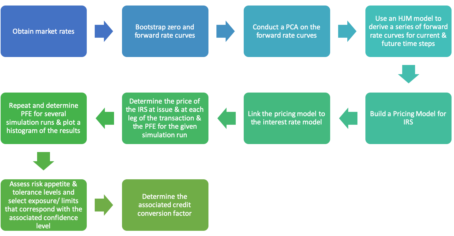
Let us take a look in greater detail at each of the steps for calculating PFE for IRS using HJM.
For the purpose of our analysis, we consider a 3 year fixed for floating interest rate swap that pays a fixed coupon every quarter of 13.50% p.a. in exchange for receiving a floating coupon equal to the 3 month Interbank Rate plus a fixed spread. The spread is 1.44%. The issue date of IRS is 19-09-2019. The coupons are exchanged at the end of each quarter, starting with the 18th day of December 2019 and continuing till maturity on 18-09-2022. The day count convention is Actual / 365. The notional amount for the transaction is Rs 100 million which is not exchanged at maturity.
Step 1: Obtain market rates
For the purpose of our analysis, we are operating in the Pakistani market and the interbank rate obtained are the KIBOR bid and offer rates for the look back period 1-January-2019 to 19-September-2019. We calculate the average of bid and offer rates to obtain our historical observed market rates.
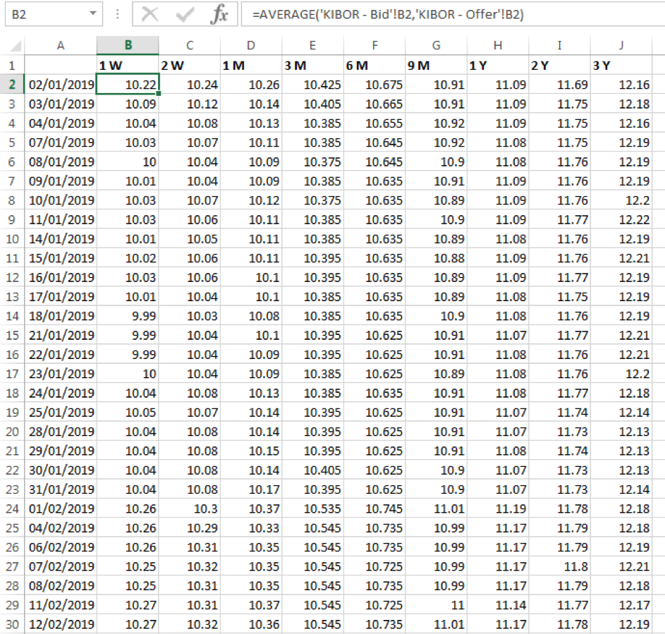
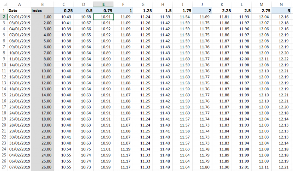
As the rates are only provided for selected tenors we use linear interpolation to derive rates for each quarter tenor from 0.25 year to 3 years.
Step 2: Bootstrap zero and forward rates from the market rates
Assuming that the market rates are for par bonds we bootstrap the interpolated interbank rates to derive zero yield curves and forward rate curves at each date. Check out the following post to review the bootstrapping methodology:
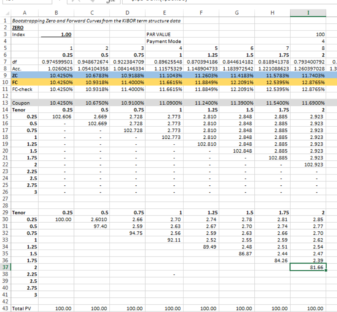
We store the results for each date in the time series in a data table:
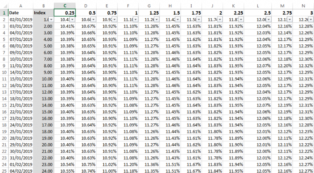
As the HJM model uses continuously compounded rates, continuously compounded zero rates are derived. Continuous forward rates are then determined from the continuously compounded zero rates.
Step 3: Conduct a PCA on the forward rates
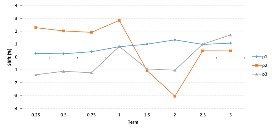
As the HJM interest rate model uses the volatility function of forward rates as an input into the model, together with the initial zero yield curve, a principal component analysis is carried on the continuously compounded forward rates derived. For our analysis, we select three factors that explain 88.78% of the volatility in the forward rates. These principle factors are depicted in the graph below:
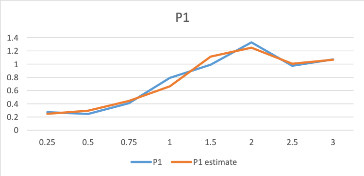
A curve is fitted to each factor using a least squares estimation process. For example, the estimated functional form for P1 (Factor 1) is shown below against the observed values:
Finally, as the factors only represent 88.78% of the total observed volatility, they are scaled so that they are calibrated to the total observed volatility.
Step 4: Derive forward rate curves using the HJM model
Using the initial zero curve yield rate, the functions for the principle factors of volatility and relevant scaling, together with random shocks applied to these factors, a forward rate curve is derived for each relevant time step in the future.
To review how to conduct a PCA, determine the main factors that explain the volatility in the underlying interest rate term structure and build an HJM interest rate model see the post below:
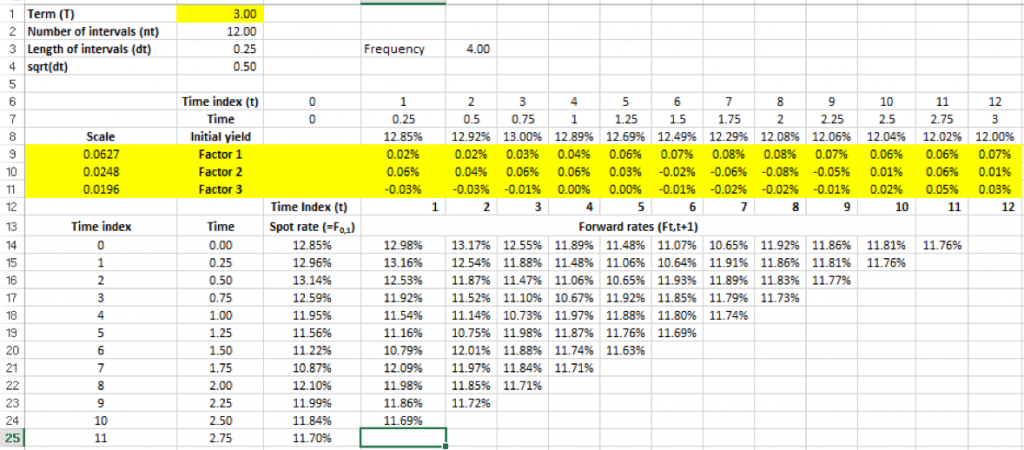
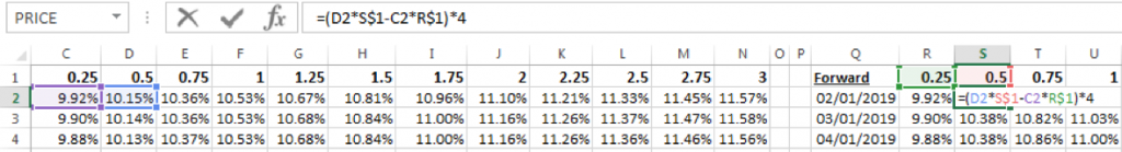
Using these forward term structures we can then determine the zero curve that will be applicable for each time step in the future:
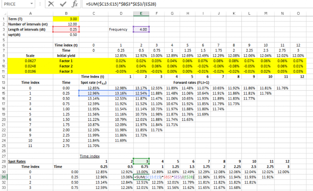
Step 5: Build a pricing model for the interest rate swap
The next step in calculating PFE for IRS using HJM is to build a pricing model for the interest rate swap. To review how to price interest rate swaps see the post below:
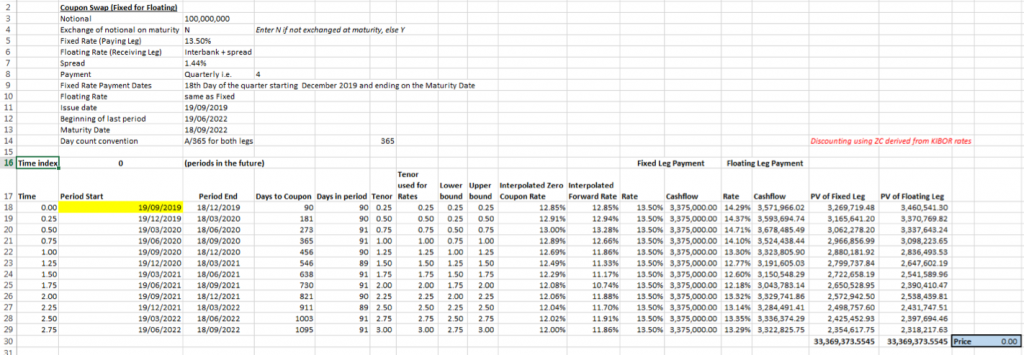
If the model is being built within an EXCEL spreadsheet, particularly one that is macro free, a separate pricing model will need to be built for each point in the time index and the IRS will be priced at that time. For our illustration, this is at issue and at each subsequent swap payment/ receipt leg.
Step 6: Link the IRS pricing model with the HJM interest rate model
The pricing model and the interest rate model are linked through the zero curve that is used to price the IRS at the specified time index. Forward rates are derived from the zero curves. For each time index, the relevant simulated zero curve structure from the HJM derivation is used.
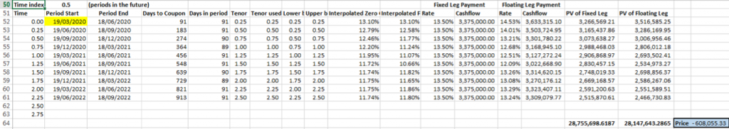
Step 7: Determine the time series of IRS prices & the PFE for a given simulation run
Over the life of the swap, determine its value (price) at issue and at each swap leg. For example, the figure below shows, for a given simulation run, the prices across the IRS’ life for the entity and its counterparty:
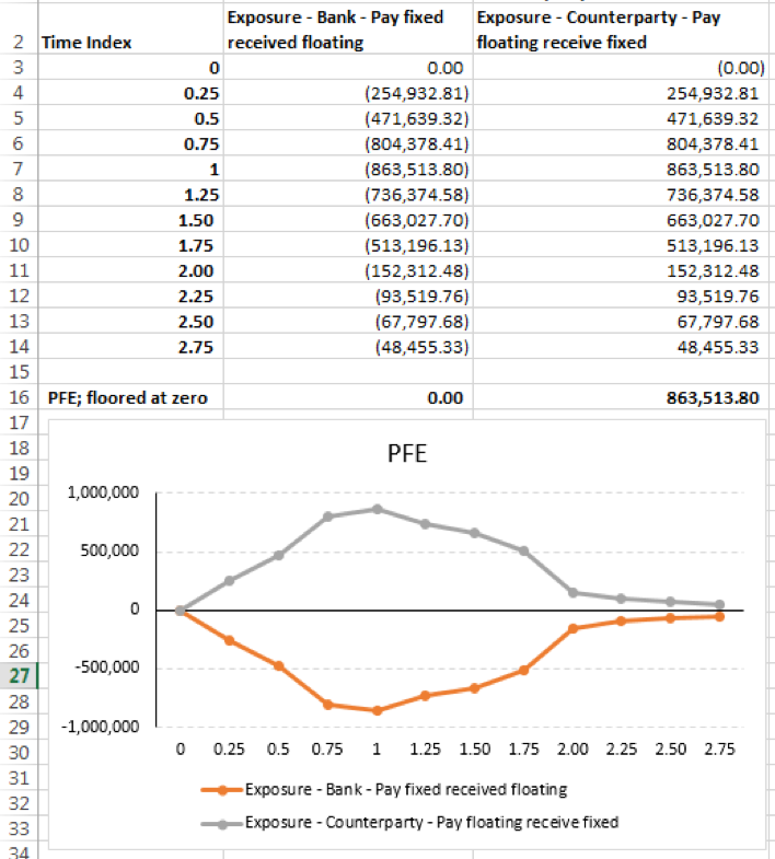
The PFE for the simulation run, is the maximum positive exposure across the time index. For the bank entity, it is null, whereas for the counterparty it is Rs 863,513.80.
Step 8: Repeat for several simulation runs and record results in a histogram
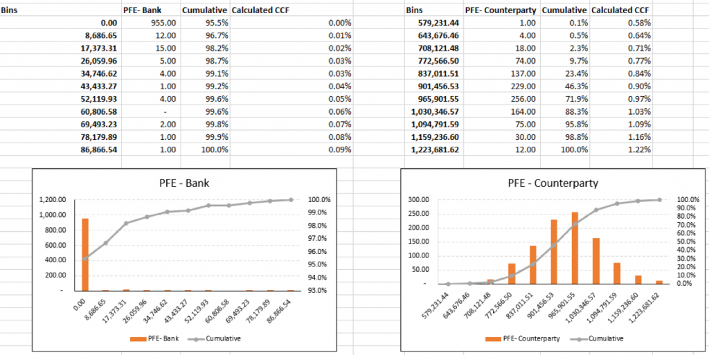
Generate the PFE in a similar manner for a number of simulation runs. In our example, we have used 1000 runs. The resulting simulated PFEs are recorded and plotted in a histogram. The distribution of results for the entity and its counterparty are as follows. In addition to the frequency distribution across value bins the cumulative frequency is calculated. This represents the probability that an exposure will be less than equal to the stated upper bound in the bin range:
Step 9: Assess risk tolerance level and select exposure/limits that correspond with the associated confidence level
Worst case PFE is approximately Rs 87,000 for the bank, while for the counterparty it is Rs 1.2 million.
In calculating PFE for IRS using HJM we need to consider the PFE distribution above, the entity’s risk appetite and tolerance level. There is 0.2% chance, or 2 days in a 1000, that the entity will face exposures in excess of Rs 70,000 while from the counterparty’s perspective there is a 30% chance, or 281 days in a 1000, that they will face exposures in excess of Rs 1 million. Each counterparty’s exposure distribution & risk tolerance will dictate the limits used by them.
Step 10: Determine the credit conversion factor
For the given PFE the credit conversion factor equals the PFE amount divided by the Effective Notional Amount. For worst case PFE the calculated credit conversion factors for the entity and its counterparty are 0.09% and 1.22% respectively.