In this course, we review the step-by-step methodology for building a three factor HJM model in EXCEL.
A pre-requisite to building the HJM model is to first determine the factors or components that will be used in the model. These factors are decided on by carrying out a principal component analysis (PCA) on the underlying term structure of interest rates.
Principal Component Analysis

Step 1 – Obtain and adjust data:
Step 2 – Construct the covariance matrix of the differences between consecutive rates in the time series:
Step 3 – Set up the calculation cells for the eigenvector matrix and its inverse
Step 4 – Define the diagonal matrix:
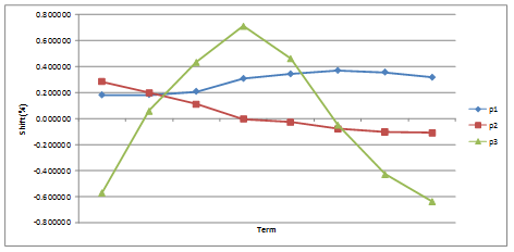
Step 5 – Tie all elements together by setting up the solver function. Run the solver function and view the resulting eigenvectors and eigenvalues. Agree on the degree of explanation that is needed with respect to the variance of the term structure and using the eigenvalue results determine the number of principal components (PCs) that would satisfy this level of explanation. Determine the functional forms of the PCs chosen and calibrate the scaling factors of these functions to the volatilities inherent in the underlying return series on the calculation date:
There are certain instances where because of the limitations of EXCEL’s Solver function a feasible result may not be arrived at. In these cases some manipulation is needed to force Solver to calculate the eigenvectors/ values:
After determining which principal components to focus on we come to the actual construction of the HJM model.
HJM Interest Rate Model
Step 1- Define the input cells including the initial zero-curve yield rates, the volatility functions derived using the principal component analysis and scaling factors to calibrate these functions, the tenor of the instrument, number and length of the time intervals:
Step 2- Next set up the calculation cells. These include calculating Brownian shocks that are applied to the volatility factors, drifts, and the spot and forward rates matrix:
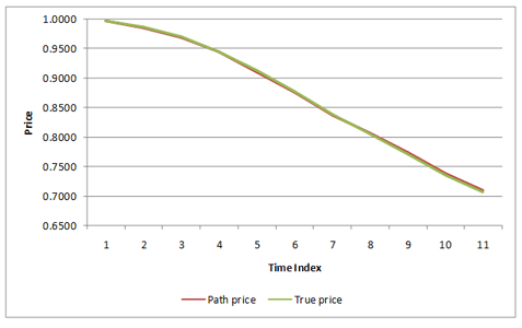
Step 3- Finally construct the output cells which give the price matrix and the path and true prices:

